Overview of data assimilation methods
Gregory J. Hakim1, J. Annan2, S. Brönnimann3, M. Crucifix4, T. Edwards5, H. Goosse4, A. Paul6, G. van der Schrier7and M. Widmannv8
We present the data assimilation approach, which provides a framework for combining observations and model simulations of the climate system, and has led to a new field of applications for paleoclimatology. The three subsequent articles explore specific applications in more detail.
Data assimilation involves the combination of information from observations and numerical models. It has played a central role in the improvement of weather forecasts and, through reanalysis, provides gridded datasets for use in climate research. There is growing interest in applying data assimilation to problems in paleoclimate research. Our goal here is to provide an overview of the methods and the potential implications of their application.
Understanding of past climate variability provides a crucial benchmark reference for current and predicted climate change. Primary resources for deriving past understanding include paleo-proxy data and numerical models, and studies using these resources are typically performed independently. Data assimilation provides a mathematical framework that combines these resources to improve the insight derivable from either resource independently. The three articles that follow describe the current activity in this emerging field of study: transient state estimation (Brönnimann et al., this issue), equilibrium state estimation (Edwards et al., this issue), and paleo data assimilation for parameter estimation (Annan et al., this issue). Here we provide an overview of these methods and how they relate to existing practices in the paleoclimate community.
In weather prediction, data assimilation uses observations to initialize a forecast (Lorenc 1986; Kalnay 2003; Wunsch 2006; Wikle and Berliner 2007). Since the short-term forecast typically starts from an accurate analysis at an earlier time, called the prior estimate, the model provides relatively accurate estimates of the weather observations. Data assimilation involves optimizing the use of these independent estimates to arrive at an analysis (i.e. estimate of the weather or climate state) with a smaller error than the model short-time forecast or the observations.
 |
|
Figure 1: Schematic illustration of how the innovation is determined in data assimilation for a tree-ring example. Proxy measurements are illustrated on the left, and model estimates of the proxy on the right. The observation operator provides the map from gridded model data, such as temperature, to tree-ring width, which is used to compute the innovation. Images credit: Wikipedia. |
 |
|
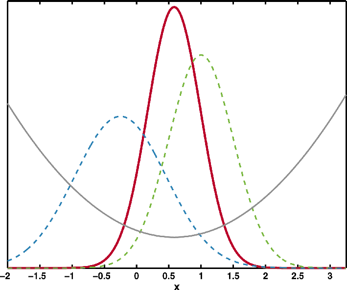
Figure 2: Data assimilation for scalar variable x assuming Gaussian error statistics. Prior estimate, given by the dashed blue line, has mean -0.25 and variance 0.5. Observation y, given by the dashed green line, has mean 1.0 and variance 0.25. The analysis, given by the thick red line, has mean 0.58 and variance 0.17. The parabolic gray curve denotes a cost function, J, which measures the misfit to both the observation and prior; it takes a minimum at the mean value of xa. From Holton and Hakim 2012. |
For Gaussian distributed errors, the result for a single scalar variable (singly-dimensioned variable of one size), x, given prior estimate of the analysis value, xp, and observation y is
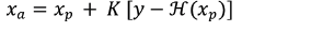 (1)
(1)where xa is the analysis value. The innovation, , represents the information from the observation that differs from the prior estimate. This comparison requires a “conversion” of the prior to the observation, which is accomplished by
  . For example, in a paleoclimate application,
 may estimate tree-ring width derived temperature data from a climate model (Fig. 1).
The weight applied to the innovation is determined by the Kalman gain, K,
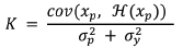 (2)
(2)where cov represents a covariance. The error variances associated with the observation and the prior estimate of the observation are given by σp and σy, respectively. Equation (1) represents a linear regression of the prior on the innovation (the denominator of K is the innovation variance). Equivalently, the Kalman gain weights the innovation against the prior, resulting in an analysis probability density function with less variance, and higher density, than either the observation or the prior (Fig. 2, red solid line, dashed green line and dashed blue line respectively). Generalizing (1) and (2) to more than one variable is straightforward, with scalars becoming vectors and variances becoming covariance matrices (for details see Brönnimann et al., this issue). These covariance matrices provide the information that spreads the innovation in space and to all variables through a Kalman gain matrix.
Application of data assimilation to the paleoclimate reconstruction problem involves determining the state of the climate system on the basis of sparse and noisy proxy data, and a prior estimate from a numerical model (Widmann et al. 2010). These data are weighted according to their error statistics and may also be used to calibrate parameters in a climate model (Annan et al. 2005).
Relationship to established methods
While there are similarities between the application of data assimilation to weather and paleoclimate, there are also important differences. In weather prediction, observations are assimilated every 6 hours, which is a short time period compared to the roughly 10-day predictability limit of the model. However, transient state estimation in paleoclimatology involves proxy data having timescales of years to centuries or longer, which generally exceeds the predictability of climate models, which are on the order of a decade. Consequently, relative errors in the model estimate of the proxy are usually much larger in paleoclimate applications. Hoever, data assimilation reconstruction may still be performed, at great cost savings, since the model no longer requires integration and each assimilation time may be considered independently (Bhend et al. 2012).
Paleoclimate data assimilation attempts to improve upon climate field reconstructions that use purely statistical methods. One well-known statistical approach for climate field reconstruction (Mann et al. 1998; Mann et al. 2008) involves limiting field variability to a small set of spatial patterns that are related to proxy data during a calibration period. Data assimilation, on the other hand, retains the spatial correlations for locations near proxies, which may be lost in a small set of spatial patterns, and also spreads information from observations in time through the dynamics of the climate model. Another distinction between data assimilation and field reconstruction approaches concerns the observation operator,  , which often involves biological quantities of proxy data that have uncertain relationships to climate. Statistical reconstructions directly relate proxy data to the set of spatial patterns, which is essentially an empirical estimate of the inverse of , and therefore subject to similar uncertainty.
Current and future directions
Research on paleoclimate data assimilation is rapidly developing in many areas. For climate state estimates, a wide range of methods are currently under exploration (see Brönnimann et al., this issue), including nudging climate models to large-scale patterns derived from proxy data (Widmann et al. 2010), and variational (Gebhardt et al. 2008) and ensemble approaches (Bhend et al. 2012). Ensemble approaches involve many realizations of climate model simulations, each of which is weighted according to their match to the proxy data, either in the selection of members (Goosse et al. 2006) or through a linear combination.
Among the important obstacles to progress in paleoclimate data assimilation, some challenges are generic, such as improving the chronological dating quality of proxy records and reducing the uncertainties of the paleoclimate data. Other problems are more specific to data assimilation, such as the development of proxy forward models. Moreover, proxy data typically represent a time average, in contrast to instantaneous weather observations, although solutions that involve assimilating time averages have been proposed to tackle this problem (Dirren and Hakim 2005; Huntley and Hakim 2010). Model bias is also problematic for paleoclimate data assimilation, especially for regions with spatially sparse proxy data.
While the field of paleoclimate data assimilation is still in its infancy, these challenges are all under active research. Merging climate models and proxy data has a bright future in paleoclimate research (e.g. the P2C2 program of the U.S. National Science Foundation), and it is likely that paleoclimate data assimilation will play a central role in this endeavor.
affiliations
1Department of Atmospheric Sciences, University of Washington, Seattle, USA; ghakim uw.edu
2Research Institute for Global Change, JAMSTEC, Yokohama Institute for Earth Sciences, Japan
3Institute of Geography and Oeschger Centre for Climate Change Research, University of Bern, Switzerland
4Earth and Life Institute and Georges Lemaître Centre for Earth and Climate Research, Université catholique de Louvain, Belgium
5Department of Geographical Sciences, University of Bristol, UK
6MARUM and Department of Geosciences, University of Bremen, Germany
7KNMI, De Bilt, The Netherlands
8School of Geography, Earth and Environmental Sciences, University of Birmingham, UK
selected references
Full reference list online under: pastglobalchanges.org/products/newsletters/ref2013_2.pdf
Annan J, Hargreaves J, Edwards N, Marsh R (2005) Ocean Modelling 8(1): 135-154
Bhend J et al. (2012) Climate of the Past 8: 963-976
Goosse H et al. (2006) Climate Dynamics 27: 165-184