PAGES Magazine articles
Pizer C.![]() 1,2, Howarth J.D.2 and Clark K.J.3
1,2, Howarth J.D.2 and Clark K.J.3
Linking onshore evidence of coseismic vertical deformation with offshore evidence of shaking is a powerful technique for better understanding the size, location and spatial impacts of past large earthquakes at subduction margins.
Coastal paleoearthquake records at subduction margins
Geologic evidence of coastal uplift and subsidence is commonly used to investigate the size, location and recurrence of past earthquakes along subduction margins (e.g. Clark et al. 2019). Large ruptures of the subduction interface are inferred by correlating coseismic deformation over large distances (>100 km). However, such spatial correlations are often based on temporal overlap between earthquake ages with uncertainties of >100 years, meaning that coseismic deformation may not have been synchronous (McNeill et al. 1999). That is, the same patterns of coastal uplift and subsidence could have been generated sequentially over decades by multiple smaller earthquakes.
Accurate correlation of coastal paleoearthquake evidence is further complicated by changes in preservation potential between sites and through time according to sea level and local erosion. Challenges imposed by incompleteness and large age uncertainties are compounded at complex subduction margins, such as the Hikurangi margin in New Zealand, where both upper plate faults and the subduction interface contribute to coseismic coastal deformation (Clark et al. 2019; Delano et al. 2023; Pizer et al. 2023a). Ultimately, incorrect paleoearthquake correlations can have implications for hazard preparedness because the spatial extent and age of past ruptures is used to inform the expected size and timing of future earthquakes (e.g. Nelson et al. 2021). Precise dating and careful interpretation of similarly timed paleoearthquake evidence is therefore essential for inferring synchronicity and potential source faults.
 |
Figure 1: Schematic demonstrating the expected patters of turbidite deposition if coastal coseismic deformation (uplift) was caused (A) synchronously at both sites in a single large earthquake, or (B) sequentially in multiple smaller earthquakes. Chronology corresponds to the example in figure 2. |
Developing turbidite paleoseismology
Submarine turbidites provide a proxy for past earthquakes recorded in the offshore portion of subduction margins where sediment archives are often longer and more complete than at the coast (Goldfinger 2011). Offshore, large gravity flows called "turbidity currents" transport remobilized sediment to the deep ocean where "turbidites" are deposited and preserved. Turbidity currents can be triggered by a number of processes, including gas-hydrate destabilization, storms and shaking during large earthquakes (Howarth et al. 2021).
The most robust way to rule out non-seismic triggers is to demonstrate that turbidity currents were initiated simultaneously over large areas (>100 km), since regionally synchronous triggering is unlikely to occur by coincidence (Goldfinger 2011). Usually, this is achieved by correlating event beds between cores from widely spaced, disconnected submarine distributary systems based on overlapping age ranges. Therefore, precise dating of turbidites is imperative to minimize age uncertainties and ensure that core-to-core correlations are unique (Hill et al. 2022).
Using turbidites to test for synchronicity of spatially-distributed coastal deformation
An independent test for an earthquake-related trigger for episodes of regional turbidite emplacement can be conducted by comparing turbidite ages against the coastal paleoearthquake record (Ikehara et al. 2016; Usami et al. 2018). Good agreement between the timing of events in both records indicates that turbidity currents were probably initiated by ground shaking during the same earthquakes that produced coseismic coastal deformation. Integrating the spatial information from both proxies can therefore help to reconstruct the extent of past earthquakes. In particular, the combined approach provides an opportunity to test the synchronicity of correlated coastal deformation by examining the number of turbidites deposited in each distributary system within the timeframe of onshore earthquake-age uncertainty (Fig. 1). For example, if a single large earthquake caused widespread synchronous deformation at the coast, we would expect to observe a single turbidite event bed in multiple submarine distributary systems (Fig. 1a). However, if multiple smaller earthquakes caused local deformation at different coastal sites within a few decades, we would expect to observe multiple turbidites offshore (Fig. 1b).
We tested the hypothesis in figure 1 with an example from the central Hikurangi subduction margin, New Zealand (Fig. 2), where two coastal sites ca. 100 km apart record similarly timed coseismic deformation. In southern Hawke’s Bay, coastal sediments from Pākuratahi display an abrupt change from estuarine silt to forest peat (Fig. 2d), indicating rapid sea-level fall, interpreted as coseismic uplift at 3630–3564 cal yr BP (Pizer et al. 2023a; Fig. 2c). In northern Hawke’s Bay, coseismic uplift of a marine terrace at Māhia Peninsula is dated to 3636–3468 cal yr BP (Berryman et al. 2018; Fig. 2c). The earthquake ages are uniquely well-constrained due to stratigraphic evidence of the precisely dated Waimihia tephra isochron, deposited decades after the earthquake (Pizer et al. 2023b). Independent of the overlapping ages, the simplest explanation for coseismic uplift at both sites is earthquakes on nearby upper plate faults. Pākuratahi was recently uplifted by ca. 2 m in the 1931 CE moment magnitude (Mw) 7.4 Napier earthquake (Hull 1990), so similar earthquakes on the Awanui fault could generate comparable vertical deformation. No historical earthquakes have occurred on the Lachlan fault, but coseismic uplift of the Māhia Peninsula has been demonstrated in elastic dislocation models (and repeatedly in the paleorecord; Berryman et al. 2018).
Offshore, sediment cores containing Holocene sequences of submarine turbidites and hemipelagic background sediment were collected from discrete distributary systems along the central Hikurangi margin (Barnes et al. 2017; Fig. 2b). Correlation between the cores is facilitated by the same macroscopic Waimihia tephra isochron identified onshore (Pizer et al. 2023b). In all cores there is a single turbidite directly beneath the tephra layer (e.g. Fig. 2e). Three cores from the Madden Canyon and Omakere distributary systems were selected for high-resolution, sequential radiocarbon dating and age-depth modeling which produced turbidite ages closely matching the coseismic uplift at Pākuratahi and Māhia Peninsula (Fig. 2c).
 |
Figure 2: (A) Location of the Hikurangi (Hik.) margin off the east coast of the North Island, New Zealand, and (B) central section spanning Hawke’s Bay (HB) with faults and paleoseismic sites. Green dots are coastal sites Māhia Peninsula (Berryman et al. 2018) and Pakuratahi (Pizer et al. 2023a). Black dots are submarine turbidite cores. Yellow dots are cores from Madden Canyon and Omakere distributary systems (Barnes et al. 2017), dated in Pizer et al. (2023b). Yellow arrows represent the flow direction of turbidity current pathways. The dotted line represents the boundary between catchments. (C) Modeled age probability density functions (PDFs) for correlated turbidites offshore and coseismic uplift onshore. (D) Evidence for coseismic uplift at Pakuratahi and (E) turbidites in the Omakere and Madden Canyon (as X-ray computed tomography (CT) scans). |
Together, the upper-slope source areas for turbidity currents in the Madden Canyon and Omakere distributary systems span northern and southern Hawke’s Bay (Fig. 2). As a result, we would expect to see multiple turbidites if separate earthquakes were responsible for generating the similarly timed deformation at Pākuratahi and Māhia Peninsula. Since we only observe a single turbidite offshore, we suggest that the coastal deformation at both sites was caused by a single earthquake. The extent of synchronous deformation (and shaking) across >100 km indicates a large magnitude earthquake which probably involved many upper plate faults rupturing together. This style of multi-fault rupture has not previously been considered in Hawke’s Bay due to the large stepovers between faults (Fig. 2b). However, as seen for the 2016 Mw 7.8 Kaikōura earthquake on the southern Hikurangi margin (Wang et al. 2018), slip on the subduction interface can help to propagate rupture across seemingly disconnected upper plate faults. The new insights from our integrated onshore–offshore paleoearthquake evidence highlight a need to incorporate complex rupture scenarios within seismic-hazard models and planning for future earthquakes on the central Hikurangi margin.
Summary
Correlating paleoseismic evidence across multiple sites is fundamental for deciphering the spatial extent and source faults for past earthquakes so that future hazard can be accurately assessed. Earthquake age-uncertainties within coastal deformation records are often too large to make unique correlations to confirm synchronous coseismic deformation. Offshore, the same events can be recorded by seismically-triggered submarine turbidites which, if carefully dated and correlated between multiple discrete distributary systems, can aid interpretation of coastal paleoearthquake evidence. For periods where regional turbidite-triggering coincides with coseismic deformation, the number of turbidites can indicate whether correlated coastal evidence represents multiple smaller earthquakes, or one larger one. Using an example from the central Hikurangi margin, we demonstrate the novel perspective provided by integrating onshore and offshore proxies, which has helped to link evidence of coastal uplift at sites separated by >100 km, to a single earthquake. Where possible, the same approach should be developed at other subduction margins to more robustly estimate the size, recurrence and source of past earthquakes.
affiliations
1Department of Geology, University of Innsbruck, Austria
2School of Geography, Environment and Earth Sciences, Victoria University of Wellington, New Zealand
3GNS Science, Lower Hutt, New Zealand
contact
Charlotte Pizer: charlotte.pizer@uibk.ac.at
references
Barnes PM et al. (2017) National Institute of Water and Atmospheric Science, 385 pp
Berryman K et al. (2018) Geomorphology 307: 77-92
Clark KJ et al. (2019) Mar Geo 412: 139-172
Delano JE et al. (2023) Geochem Geophys Geosyst 24: e2023GC011060
Goldfinger C (2011) Annu Rev Mar Sci 3: 35-66
Hill JC et al. (2022) Earth Planet Sci Lett 597: 117797
Howarth JD et al. (2021) Nat Geo 14: 161-167
Hull AG (1990) New Zealand J Geol. Geophys 33: 309-320
Ikehara K et al. (2016) Earth Planet Sci Lett 445: 48-56
McNeill LC et al. (1999) Geol Soc Spec Publ 146: 321-342
Nelson AR et al. (2021) Quat Sci Rev 261: 106922
Pizer C et al. (2023a) GSA Bulletin
Pizer C et al. (2023b) Quat Sci Rev 307: 108069
Kleemann K.![]()
New England has the longest continuous earthquake record in the United States. Earthquake catalogs document the exact time that an earthquake struck. When consulting historical sources, however, it becomes clear that there is much more ambiguity concerning these documented times.
Earthquakes in New England
Earthquakes that took place during historical times are often recorded in historical documents. Where earthquakes are infrequent, they are perceived as something extraordinary and are remarked upon as such in diaries, letters, newspapers, and sermons. A list of regions in the United States that evoke associations with earthquakes include California, Alaska and Washington. New England does not necessarily spring to mind. However, despite being located on a tectonic plate, some distance away from the active continental margins, earthquakes do occur there. These seismic events are called intraplate earthquakes.
 |
Figure 1: A page of Cotton Tufts’ annotated almanack showing his entry for an earthquake on 29 November 1783 CE (see black arrow). Photography by the author. Credit: Cotton Tufts’ diary, 29 November 1783 CE, Collection of the Massachusetts Historical Society. |
The seismic activity in this region is caused by the repercussions of the ancient collision between the African continent and the North American continent, which formed the supercontinent Pangea 450 to 250 million years ago, and the subsequent breakup of Pangea, which formed the Atlantic Ocean. Today’s fault lines are echoes of these events in deep geological time (Kafka 2004). Some of these fault lines are occasionally reactivated by stress caused by the movement of the North American plate, moving away from the mid-Atlantic ridge, and by postglacial rebound, which is an uplift of a tectonic plate formerly weighed down by thick sheets of ice during an ice age; in this case, the ice sheets that started to melt around 10,000 years ago (Natural Resources Canada).
In North America, earthquakes to the east of the Rocky Mountains are felt in a much larger geographic area than those to the west. Indigenous peoples residing in North America experienced earthquakes here for a long time and passed on knowledge about them through oral history. Settlers arriving from Europe in the 17th century started recording them in written form after their arrival. In annotated almanacks, for instance, we can see that locals recorded when they felt the "small shock of an earthquake" (Fig. 1). The Massachusetts-based physician, Cotton Tufts, wrote that particular entry about an earthquake on 29 November 1783 CE that originated in northern New Jersey and was felt across New England (Kleemann 2018). Early American residents of the northeastern parts of the country, unlike modern residents, did not regard earthquakes as "such an anomaly" (Robles 2017).
Notable earthquakes felt in New England (Fig. 2) originated in New Hampshire in 1638 CE; in Newburyport, Massachusetts, in 1727 CE; off the coast of Cape Ann near Boston in 1755 CE; in Moodus, Connecticut, in 1791 CE; in New York City in 1884 CE, in New Hampshire in 1940 CE; and in Virginia in 2011 CE.
Earthquakes put early American timekeeping practices to the test
The above-mentioned earthquakes are listed in earthquake catalogs. In addition to the approximate magnitude and intensity, these listings also include information on the date and time of the earthquake. Today, this is common practice and relatively easy to reconstruct, as a network of hundreds of seismographs around the world are recording earthquakes near and far. Seismographs were only invented in the late 19th century (Coen 2012). Seismographic records for New England date back to 1900 CE (Ebel et al. 2020). Older earthquake catalogs, however, also list precise times for those earthquakes that took place before the invention of the seismograph.
 |
Figure 2: A map showing the assumed epicenters of selected earthquakes that affected New England over the past four centuries. The abbreviations on the map refer to the American states and Canadian provinces (NJ refers to New Jersey, QC to Quebec, etc.). Artwork credit: Jack Walsh, used with permission. |
One problem that can arise, when considering the timing of historical earthquakes in this period, is the apparent discrepancy between the dates documented across certain borders. This occurs because some regions at the time still used the Julian calendar, whereas other regions had already adopted the Gregorian calender, which was first introduced in 1582 CE as a modification of the Julian calendar. In historical earthquake catalogs, this has sometimes led to confusion and incorrect listings. For instance, the geologist William T. Brigham listed 26 January 1662 CE and 5 February 1663 CE as separate earthquakes in his Historical Notes on the Earthquakes of New England; however, they are one and the same event. This earthquake was felt widely and originated in La Malbaie, New France, today’s Canada; a Catholic area that used the Gregorian calendar while the American colonies were still using the Julian calendar (Brigham 1871; Ebel 1996). In New France, the new year began on 1 January, whereas it only began on 25 March in New England. January was considered part of 1662 CE in New England and 1663 CE in New France; this observation explains the huge discrepancy in recorded dates and the subsequent mix-up by Brigham (1871).
The most specific time listed for an early modern earthquake in the United States Earthquake Intensity Database (United States Geological Survey 1986) catalog is for the 1755 CE Cape Ann earthquake. The time given for the event is 4:11:35 a.m. How was such a precise time recorded? In 1620 CE, the Mayflower ferried pilgrims across the Atlantic without a single timepiece on board (Hering 2009). At first, little metal was available in the New World, which made it challenging to produce clocks locally. Therefore, settlers began bringing timepieces with them from Europe, starting in 1650. Towers of churches, town hall, and other public buildings also began to install clocks around the same time (Distin and Bishop 1976). By 1700 CE, every colony had clockmakers (O’Malley 1990). The clocks available in the 17th and 18th centuries needed to be wound up regularly to run. Over time, as would be expected, the clocks in the New World improved (Distin and Bishop 1976).
Clocks were relatively expensive, only becoming more affordable and accessible toward the end of the 18th century with the beginning of mass production. Before this, it was mostly merchants, professionals, and shopkeepers who owned clocks and watches. Townspeople were more likely to have access to timepieces than those in the country (O’Malley 1990).
Coming back to the question of precise timing of the 1755 CE earthquake, John Winthrop, a professor at Harvard College, had found that one of his clocks had stopped precisely at 4:11:35 a.m (Winthrop 1755). For the purpose of another experiment, he had previously placed an item inside his clock’s case, which had dislodged during the earthquake and fell against the pendulum inside the case, thereby stopping the clock. When consulting the sources, however, it becomes apparent that many other times when the 1755 CE Cape Ann earthquake allegedly struck are available, ranging from 3 to 5 a.m. While Winthrop, as a professor and person of science, likely took good care of his clocks, it should still be considered as one reading among many. It remains impossible to know precisely when the earthquake occurred.
Earthquakes and timekeeping from the 19th century onward
Before the widespread use of railroads made the standardization of time zones necessary, the local time of a given town was set when the sun crossed the meridian. Every town had its own time zone, slightly different from those towns to the east and west (Bartky 2000). While travel during this time was slow, measured in days rather than hours and minutes, the almost instantaneous spread of an earthquake’s waves put timekeeping practices to the test. In 1883 CE, delegates from the US railroads adopted the Standard Time System, which was officially recognized by the passing of the Standard Time Act by the US Congress in 1918 CE (Olmanson 2011). Today, towns no longer observe their own time zones based on solar time. Not only does this make communication and transportation more practical, but it also makes recording earthquakes around the globe easier.
ACKNOWLEDGEMENTS
The author thanks the John Carter Brown Library for a fellowship in 2020–2021 that allowed her to research the library’s collections for this project.
affiliation
German Maritime Museum / Leibniz Institute for Maritime History, Bremerhaven, Germany
contact
Katrin Kleemann: k.kleemann@dsm.museum
references
Ebel JE (1996) Seismol Res Lett 67: 51-68
Ebel JE et al. (2020) Seismol Res Lett 91: 660-676
Hering DW (2009) Accessed 5 Dec 2023, collectorsweekly.com
Kafka AL (2004) accessed 5 Dec 2023, aki.bc.edu
Kleemann K (2018) accessed 5 Dec 2023, envhistnow.com
Natural Resources Canada (website), accessed 5 Dec 2023
O’Malley M (1990) Keeping Watch: A History of American Time. Viking, 384 pp
Robles WB (2017) The New England Quarterly 90: 7-35
United States Geological Survey (website), accessed 5 Dec 2023, ncei.noaa.gov
Lallemand T.![]() 1, Audin L.
1, Audin L.![]() 2, Quiquerez A.
2, Quiquerez A.![]() 1, Baize S.
1, Baize S.![]() 3, Grebot R.2 and Mathey M.
3, Grebot R.2 and Mathey M.![]() 3
3
A multidisciplinary study combining structural geology, geomorphology and archaeoseismology on a Gallo-Roman site in the Jura Mountains shows potential evidence of recent tectonic deformation along the northern Montagne du Vuache Fault. These new findings question the role of past earthquakes in the site abandonment.
Seismotectonic background of the Montagne du Vuache Fault (MVF)
The MVF is a major fault system extending over ~80 km from the edge of the Alpine range to the Jura Mountains (calcareous rocks), through the southernmost Swiss Molasse basin (sandstones and siltstones, Baize et al. 2011; Fig. 1). The recent tectonics of the MVF have been studied in its southeastern part, following the damaging Epagny earthquake near Annecy (13 July 1996; moment magnitude [Mw] 4.8; Thouvenot et al. 1998; Courboulex et al. 1999; Fig. 1a).
While Quaternary left-lateral faulting has been confirmed there (e.g. displacement of small valleys, syn-depositional deformation, Baize et al. 2011; De La Taille 2015), these studies have not yet demonstrated the occurrence of surface-rupturing events during the last thousands of years. Tracking those surface-rupture events is crucial to defining the seismic hazard related to the fault. This can be achieved by dating deformed features, either on natural or anthropogenic objects.
As the fault extends northwestward into the Jura Mountains, it splits into multiple segments. In this area, the youngest evidence of fault activity at the surface relies on syntectonic mineralized calcites, the dating of which indicates a main phase of activity at around 10 Ma followed by a reactivation phase at ~5 Ma (Smeraglia et al. 2021).
 |
Figure 1: (A) Geomorphological imprint of the fault based on a 5 m spatial resolution DEM, and on a 25 cm spatial resolution DEM in the boxed area. (B) Calcite steps observed on a fault plane, here with left-lateral strike-slip kinematics. (C) Example of left-lateral offset across limestones along one of the main fault segments. Projected coordinate system: EPSG 2154, RGF93 / LAMBERT 93. |
What’s new along the northern section of the MVF? A morphotectonic and structural perspective
We analyzed the geomorphological imprint of the fault, based on a regional 5 m spatial resolution Digital Elevation Model (DEM), as well as a 25 cm spatial resolution DEM around the Villards d’Héria area (black square in Fig. 1a), to identify geomorphic markers (lineaments, surface fractures, watercourses, limestone beds, ridge lines, valley bottoms, and geological units), revealing horizontal displacements.
Along the MVF trace running from Annecy to the Jura Mountains, we detected 342 lineaments (Fig. 1a). About 45% of them were identified as fault segments, showing signs of kinematics, with 75% of them exhibiting left-lateral motion (red segments, Fig. 1a), predominantly in the NW-SE direction. Segments with other orientations and kinematics may be old inherited faults, or secondary faults conjugated to the main faults (black segments, Fig. 1a).
As suggested by the potentially active fault map of France (Jomard et al. 2017), the MVF signature in morphology splits as it reaches the Jura mountain range, with one section crossing the area of interest around Villards d’Héria, suggesting that the distribution of the deformation is controlled by surface lithology. Where "hard" rocks (limestones) are close to the surface, the subparallel segments are numerous (Jura domain, NW part of the fault). Conversely, fault segmentation is limited, and the geometry appears rather continuous where "soft" rocks (molasse) are dominant (Savoy area, southeastern part of the fault). A splay fault structure can thus be observed in our study area, which is located at the northwestern end of the MVF (Fig. 1a). Numerous fault segments can be observed in the morphology there (Fig. 1a). Field investigations confirmed numerous NW-SE fault planes with left-lateral, strike-slip kinematics, evidenced by calcite steps (Fig. 1b). When associated with their conjugate faults (right-lateral, NE-SW), the paleostresses accommodated by these faults can be well constrained.
A preliminary slip rate was estimated from limestone bed offsets (Fig. 1c), based on the analysis of the lineaments detected on the DEM. The displacement classification shows that the most represented classes occur between 200 m and 1000 m of cumulative horizontal displacement. Smeraglia et al. (2021) proposed that the first phase of deformation occurred at 10 Ma (onset of Jura NW-SE shortening), and that a second phase occurred at around 5 Ma, with corresponding slip rates between 0.02-0.1 mm/yr and 0.04–0.2 mm/yr, respectively. These values fall in the lower range of the slip rates proposed by Baize et al. (2011) based on regional correlations.
The Gallo-Roman site and the potential for archaeo-earthquakes
The sanctuary area of Villards d’Héria provides the ideal archaeological context for studying the cause-and-effect relationship between a faulted bedrock and deformation of archaeological remains. The sanctuaries are spread over two sites (Fig. 1c). The upper site, near Lake d’Antre (802 m asl) is bounded by the Antre Fault. The lower site, "Pont-des-Arches", in the Héria Valley (712 m asl) consists of a worship area and bathing facilities. The two sites are connected by karstic conduits (Nouvel et al. 2018), whose flow is driven by a dense fracture network. Excavations have provided evidence of continuous occupation from the first century BCE until the last decades of the third century.
 |
Figure 2: Area of archaeoseismological investigations. (A) Zenithal view of deformed walls, and (B) structural diagram of the faulted zone, and impacted infrastructures. (C) Focus (red box on (B)) on Wall 2 displaying two phases of damage: a sinistral offset at the base (phase 1), and a tilting of the structure in the upper part (phase 2). |
In 2021, while conducting excavations at the lower site, unexpected signs of damage and disorders were identified on the archaeological remains, specifically on walls (Wall 1 and Wall 2, Fig. 2). Further exploratory field surveys in 2023 revealed that the archaeological deformation features were collocated with left-lateral kinematics in the bedrock. The facing of the two walls displays obvious misalignments, visible in both plan and zenithal views (Fig. 2b). At this point, Wall 1 exhibits a minimum left-lateral offset of 10 cm, taking the wall orientation without deformation as reference. Deformation features on Wall 2 potentially imply two phases of deformation. The base of the wall is left-laterally shifted with an offset of 25 cm (phase 1), assuming an initial straight shape when it was built (indicated by the green line, Fig. 2c). Some of the blocks are broken, and a mortar was used to reinforce this part of the wall, which could have been used then as a foundation of the upper wall. Later, this latter wall was tilted (phase 2), dipping 70° to the east (Fig. 2c). All the Roman remains are sealed by a backfill layer, from the early third century. The disorders observed on the walls, and the geological deformation features observed in the bedrock, are consistent with each other and with regional observations. The sinistral displacements observed on the walls could be the result of one or more ruptures during an earthquake(s) on a segment of MVF faults that needs to be further investigated.
Quantifying deformation through 3D reconstruction of the archaeological remains
At locations where the remains are well preserved, we plan to quantify deformations at a subcentimeter and millimeter scale on geological and archaeological markers through a detailed analysis of ortho-images and a high-resolution Digital Surface Model. This approach will facilitate the systematic examination of disorders, linear and/or angular deformations, and their comparison, by juxtaposing surveys a few meters apart. We also need to check the kinematic consistency of different archaeological markers at the archaeological site scale, to confirm the surface-rupture hypothesis.
Paleoseismological investigation
To better assess the tectonic history of the MVF, we intend to conduct a statistical analysis of striation orientations, coupled to dating of kinematic markers (U-Pb or U-Th, depending on their age). In addition, to enrich the timing of surface-rupturing events, we will perform a twofold paleoseismological investigation. We will focus on: 1) examining the stratigraphic records in the lacustrine sediments of Lake d’Antre, which is bounded by a MVF segment to the south (Fig. 1c); and 2) trenching across fault scarps to unearth rupture traces in the Holocene sediments and soils. These two datasets will, we hope, enable us to complete the chronology by going back in time, covering (partly) the Holocene. A set of sediment cores was already retrieved from the lake in June 2023, and their analysis is currently in progress. Concurrently, we will conduct Electric Resistivity Tomography profiles and explore prospective pits to locate suitable locations for paleoseismological trenches. We are also experimenting with subaqueous imaging techniques to investigate whether any tectonic deformation extends to the lake bottom.
The preliminary results reported here suggest the occurrence of tectonic events during Antiquity along the northern segments of the MVF. Surface-rupture faulting could have damaged and offset Gallo-roman remains, and strong local shaking during those events could have coevally damaged the constructions. If confirmed, the 20–30 cm wall offset could fit with the deformation characteristic of a shallow to very shallow moderate-magnitude earthquake, capable of causing strong shaking in the vicinity of the fault. From an archaeological point of view, this new hypothesis raises the question of the role of earthquakes on the site abandonment, whether due to the direct effects of earthquakes or their potential impact on hydrological flows in this karstic environment.
ACKNOWLEDGEMENTS
Special thanks to Vincent Bichet (Lab. Chrono-environnement, University of Franche-Comté, France) and his team for Lac d’Antre coring, and Philippe Roux and Jean Guillard (Lab. ISTerre University of Grenoble, and Lab. CARTELL, INRAE) for acoustic data acquired at Lac d’Antre. All these people are part of the ongoing effort developed to image the fault impacts on the upper site. We would also like to thank the Service Régional Archéologique of the Bourgogne-Franche Comté region, and the PCR "Villards d’Heria", for their financial support and the facilitation of this study.
affiliationS
1Université Grenoble Alpes, IRD, ISTerre, Grenoble, France
2ARTEHIS, Bourgogne University, France
3Institute for Radioprotection and Nuclear Safety, Fontenay aux Roses, France
contact
Théo Lallemand: theo.lallemand@univ-grenoble-alpes.fr
references
Baize S et al. (2011) Bull Soc Géol Fr 182: 347-365
Courboulex F et al. (1999) Geophys J Int 139: 152-160
De La Taille C (2015) PhD thesis, Université Grenoble Alpes, 259 pp
Jomard H et al. (2017) Nat Hazards Eath Syst Sci 17: 1573-1584
Nouvel P et al. (2018) Rec Archeol 32: 103-114
Smeraglia L et al. (2021) Journal of Structural Geology 149: 104381
Patria A.![]() and Daryono M.R.
and Daryono M.R.![]()
The Matano Fault in Sulawesi, Indonesia, has remained unruptured for the last two centuries. However, paleoseismic investigations reveal a seismic hazard potential as large as that of the Mw 7.5 Palu earthquake in 2018 CE.
Background
Sulawesi, Indonesia, is an actively deforming region with intense seismicity due to the rapid convergence between the Eurasian, Pacific, and Australian plates (Fig. 1; Bock et al. 2003). The most recent surface-faulting event was the 2018 CE Mw 7.5 Palu earthquake that ruptured a ~170 km long portion of the Palu-Koro Fault in central Sulawesi, and caused massive destruction in Palu City and surrounding areas (Natawidjaja et al. 2021). A question has been raised about the seismic hazard of Sulawesi. Where are the next large earthquakes (Mw ≥7) likely to occur?
The Matano Fault is the southeastern extension of the Palu-Koro Fault. This fault has the considerable capability of producing large earthquakes (Center of National Earthquake Study (PuSGeN) 2017; Watkinson and Hall 2017). The fact that no historical report about large earthquakes on the fault is available indicates that the fault has remained unruptured for at least two centuries, and has been storing enough slip (energy) to be released for the next surface-rupturing earthquakes. To date, the largest modern seismicity on the Matano Fault was the 2011 CE Mw 6.1 earthquake near Lake Matano.
The left-lateral motion in eastern Indonesia, due to the fast westward motion of the Pacific plate relative to the Australian plate, is accommodated by the Palu-Koro and Matano faults in Sulawesi (Fig. 1). The Palu-Koro Fault slips at ~ 40 mm/yr (Socquet et al. 2006) while the Matano Fault moves at ~20 mm/yr (Khairi et al. 2020; Walpersdorf et al. 1998). These motion rates are comparable to the San Andreas Fault’s motion in the US, at ~30 mm/yr (Sieh and Jahns 1984). However, limited fundamental geological information on the Matano Fault, such as history of large seismic events, the potential maximum magnitude and the extent of surface-rupturing earthquakes, has been a significant barrier to evaluating the seismic hazard posed by the fault.
 |
Figure 1: Active fault map of central Sulawesi with modern seismicity (modified from Center of National Earthquake Study (PuSGeN, 2017). Locs. 1, 2, and 3 indicate the locations of fault ruptures observed by Daryono et al. (2021), the paleoseimic trench by Patria et al. (2023), and submerged iron production settlement at Lake Matano (Adhityatama et al. 2022), respectively. Note that the 2018 Mw 7.5 earthquake’s rupture still extends further north, beyond the map. |
Recent paleoseismic investigations that examine the relationship between stratigraphy and fault structures at the shallow subsurface have revealed the seismic behaviors of the Matano Fault, which is helpful to better mitigate seismic hazards for the areas near the fault (i.e. Daryono et al. 2021; Patria et al. 2023).
Seismic behaviors of the Matano Fault
The Matano Fault traverses central Sulawesi for ~190 km in a NW-SE direction and consists of six geometric segments separated by structural discontinuities (Fig. 1). The first evidence of surface-rupturing earthquakes in the past on the Matano Fault was revealed by Daryono et al. (2021), who found evidence of two seismic events dated to ~4200–3000 BCE on the fault segment east of Lake Matano (Loc. 1 in Fig. 1). Geomorphic reconstruction by Daryono et al. (2021) also indicated a total left-lateral offset of ~400 m due to the fault motion. The Matano Fault has repeteadly moved and produced Mw 7-class earthquakes, rupturing multi-fault segments, similar to the 2018 Mw 7.5 Palu earthquake (Daryono et al. 2021).
A recent study by Patria et al. (2023) investigated the easternmost portion where the fault runs within a quaternary basin, called the Larongsangi basin (Loc. 2 in Fig. 1). Based on tectonic geomorphic interpretation using a high-resolution digital elevation model (DEM) generated from the LiDaR (Light Detection and Ranging) data, they mapped geomorphic features and surface traces of the Matano Fault. Along the fault, the smallest left-lateral offset was on the beach ridge, ~7 m, accompanied by a 1 m high fault scarp (Fig. 2). These features were interpreted as a result of a single earthquake because they were found on the youngest geomorphic surface.
Based on the scaling relations by Wells and Coppersmith (1994), the 7 m offset was likely caused by a Mw 7.4 earthquake rupturing a 110 km long fault. A paleoseismic trenching on a 2 m high fault scarp revealed the history of surface-rupturing earthquakes (Loc. 2 in Fig. 1). Using the trench observation and radiocarbon dating, the most recent surface-rupturing earthquake was dated between 1432–1819 CE. The penultimate and antepenultimate surface-rupturing earthquakes were constrained between 1411–1451 CE and 981–1355 CE, respectively. There were two other older earthquakes which occurred prior to 1000 CE. Therefore, based on the timing of these earthquakes, the reccurence interval was estimated at 335 ± 135 years.
 |
Figure 2: (A) Topographic profile and (B) photograph of the smallest fault scarp cutting the youngest beach ridge on the eastern Matano Fault. This geomorphic feature was interpreted as a result of a single surface-rupturing earthquake. |
Seismic hazard evaluation
Lake Matano in the center of the Matano fault occupies a 6 km wide stepover between two fault segments (Fig. 1). According to Wesnousky (2006), stepovers wider than 4 km behave as earthquake-rupture terminations for large earthquakes. Patria et al. (2023) postulated that the surface-rupturing earthquake observed in the paleoseismic trench (Loc. 2 in Fig. 1) spanned ~110 km from Lake Matano to the offshore east of the Larongsangi basin (Fig. 1). The absence of a surface-faulting event on the Matano Fault in the last two centuries suggests that the fault may have formed two seismic gaps, separated by Lake Matano, which are potential locations for the next surface-rupturing earthquakes.
Large seismic events on the Matano Fault could be devastating. Within Lake Matano, an iron production village dating back to the eighth century had submerged at a depth of 3–15 m (Loc. 3 in Fig. 1) (Adhityatama et al. 2022). This iron production site’s subsidence could have been caused by catastrophic events, possibly repeated large earthquakes on the Matano Fault. For the eastern portion of the Matano Fault, the elapsed time since the most recent surface-faulting event is more than 200 years, exceeding the minimum calculated recurrence interval. Thus, the next surface-rupturing earthquake is plausibly due for the eastern portion. In addition to the shaking and ground deformation, large earthquakes on the Matano Fault, particularly the eastern portion, could cause a submarine-landslide tsunami.
Structural interpretion by Titu-Eki and Hall (2020), based on high-resolution multibeam bathymetry, indicated the existence of large submarine landslides at continental slope near the fault. Such landslides could have been triggered by strong shaking, and may have generated tsunamis.
Summary
Paleoseismic studies on the Matano Fault have revealed the history of large seismic events on the fault and the magnitude and extent of surface-rupturing earthquakes, which are helpful for seismic-hazard assessment. The Matano Fault forms two seismic gaps that could produce the next large earthquakes. Studies on the Matano Fault demonstrated the benefits of paleoseismic investigation to understand the seismic hazard posed by the fault.
In Indonesia, many active faults have been identified, but geological information on these faults is still lacking. Therefore, more paleoseismic studies are required to understand the seismic behaviors and evaluate the seismic hazard of these active faults. Subaqueous paleoseismic investigations on Lake Matano may also be useful in providing a longer and more complete record of earthquakes than the conventional paleoseismic method, as demonstrated by Tournier et al. (2023) in Lake Towuti, southeast of Lake Matano.
ACKNOWLEDGEMENTS
We thank Danny H. Natawidjaja, Mohammad Heidarzadeh, Hiroyuki Tsutsumi, Muhammad Hanif and Anggraini R. Puji for the discussion of the research on the Matano Fault.
affiliation
Research Center for Geological Disaster, National Research and Innovation Agency (BRIN), Bandung, Indonesia
contact
Adi Patria: adi.patria@brin.go.id
REFERENCES
Adhityatama S et al. (2022) Archaeol Res Asia 29: 100335
Bock Y et al. (2003) J Geophys Res 108: 2367
Daryono MR et al. (2021) IOP Conf Ser Earth Environ Sci 873: 12053
Khairi A et al. (2020) J Geod Undip 9: 32-42 (in Indonesian with English abstract)
Natawidjaja DH et al. (2021) Geophys J Int 224: 985-1002
Patria A et al. (2023) Tectonophysics 852: 229762
Sieh KE, Jahns RH (1984) GSA Bull 95: 883-896
Socquet A et al. (2006) J Geophys Res 111: B08409
Titu-Eki A, Hall R (2020) Indones J Geosci 7: 291-303
Tournier N et al. (2023) Quat Sci Rev 305: 108015
Walpersdorf A et al. (1998) Geophys J Int 135: 351-361
Watkinson IA, Hall R (2017) Geol Soc Spec Publ 441: 71-120
Wells DL, Coppersmith KJ (1994) Bull Seismol Soc Am 84: 974–1002
Grützner C.![]()
Slow faults only rarely produce large earthquakes, we often know little about their past activity, and they are difficult to study. Here, I show how using a combination of different tools helps to reveal past fault-surface ruptures in Slovenia.
Slow-moving faults are difficult beasts
Faults with high slip rates of several millimeters, or even centimeters, per year can host large earthquakes with typical recurrence intervals of a few hundred years. Good examples are the Alpine Fault in New Zealand, the North Anatolian Fault in Türkiye, or the San Andreas Fault System in California (e.g. Onderdonk et al. 2018). Living in such regions comes with the obvious problem of frequent strong quakes. However, perhaps surprisingly, there is also good news: people know about the seismic hazard because the last strong event was not long ago, and they are usually prepared. Chile, for example, was struck by a subduction earthquake moment magnitude (Mw) 8.8 in 2010, yet less than 600 people lost their lives—remarkable for the sixth strongest earthquake ever measured. The same is true for Japan. Slow-moving faults, on the other hand, cause infrequent strong quakes (Liu and Stein 2016). We saw this in Morocco on 8 September 2023, when an earthquake of Mw 6.8 occurred in a region of low instrumental and historical seismicity, and tragically caused thousands of deaths. In fact, more people have been killed by earthquakes in continental interiors than by those that occurred on plate boundaries (England and Jackson 2011).
Apart from the issues with estimating the seismic hazard of areas that are slowly deforming, slow faults come with another problem: their movement often leaves only subtle traces in the landscape because it is outpaced by other processes such as erosion, sedimentation and modification by humans. Studying their tectonic activity, slip rate etc. can, therefore, be very difficult (Diercks et al. 2023; Grützner et al. 2017).
The Idrija Fault in Slovenia
In the framework of the German Priority Program "SPP2017 – Mountain Building Processes in 4D" we looked into the tectonic activity of the Alps-Dinarides junction (Fig. 1). Here, the northward motion of the Adriatic Plate of about 2–3 mm/yr, with respect to stable Europe, is accommodated by a strike-slip fault system in Western Slovenia. The system is made up of at least four major faults and several smaller ones. They strike NW–SE and are parallel to each other (Fig. 1). Seismicity is low to moderate and only one of these faults had strong instrumental earthquakes of magnitudes Mw 5.7 and Mw 5.2 in 1998 CE and 2004 CE, respectively. Swarm activity, however, has been proven for the largest faults (Vičič et al. 2019).
 |
Figure 1: Map of the study area in Slovenia. Faults (simplified) in red, the Idrija Fault in bold. Adria moves north with respect to Eurasia with 2–3 mm/yr. |
A destructive earthquake in 1511 CE devastated the city of Idrija, back then an important mercury mining town. Still, there is debate as to whether this quake occurred on the Idrija Fault, the longest fault of the system (~100 km), or on another fault in Italy (Falcucci et al. 2018; Fitzko et al. 2005). The quake’s magnitude was perhaps close to MW 7. Because of the slow motion of Adria, individual faults in our study area have low slip rates, probably not exceeding 1 mm/yr (Atanackov et al. 2021; Grützner et al. 2021; Moulin et al. 2016). This, in return, means that it may take thousands of years before enough strain is accummulated to be released in a major earthquake in which the fault slips by a meter or more, and which breaks the surface. One therefore has to go beyond the instrumental and historical record to investigate the Idrija Fault’s earthquake history.
While a few studies could prove fault activity during the Late Quaternary and estimated the slip rate, only one attempt has been made to date the last major earthquake on the fault by paleoseismological trenching—that is, excavating the fault zone and dating offset or deformed geological layers (Bavec et al. 2013). The results of this study imply that the Idrija Fault ruptured in 1511 CE. But how often do these large earthquakes happen? In order to find out, we decided to open another paleoseismological trench across the fault, but choosing the right place is not an easy task.
Combining different methods helps to reveal past earthquakes
A suitable trench site needs to fulfill a couple of prerequisites. First, there needs to be young geological units that have recorded fault motion. We therefore had to find a site with Late Quaternary sediments and constant sediment input. The idea is that dating the youngest deformed units and the oldest non-deformed units enables bracketing the date of the earthquake. Second, we need to find sediments that can actually be dated by radiocarbon, luminescence, or other methods. Third, the trench needs to hit the actual fault zone. Fourth, the logistics must work: Can I reach the site with an excavator? Is the site within a National Park? Does the landowner agree? Will I need to pump groundwater?
After mapping the fault trace using a 1 m digital elevation model created from airborne laserscanning data (ARSO 2015), we ran an extensive geophysics campaign and collected kilometers of georadar and geoelectrics profiles across the fault.
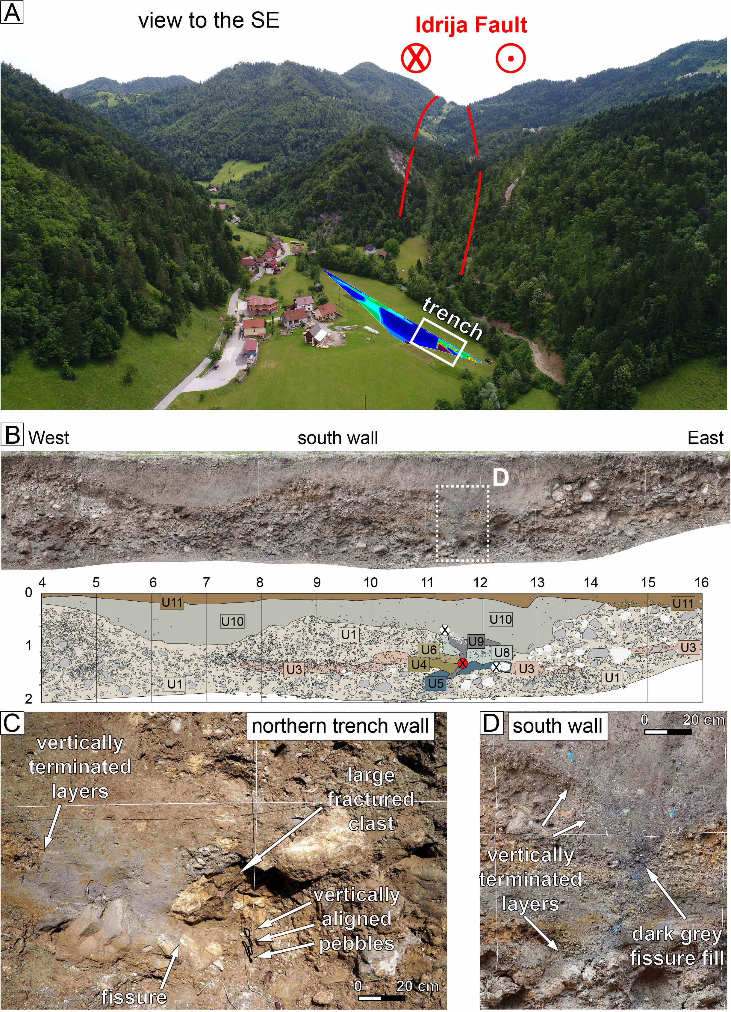 |
Figure 2: The trench site at Srednja Kanomlja, near Idrija. (A) Panoramic view of the trench site with the fault trace in the background and results of the geoelectrics measurements (blue: low resistivities; red: high resistivities). (B) Photo and 1:10 scale log of the trench wall. Circles with crosses mark sample locations for dating. (C-D) Details from the trench. |
One site fulfilled all requirements—a small basin on the fault trace with a strong contrast of resistivities in the subsurface (Fig. 2a). This contrast indicates that two different types of rocks are juxtaposed, in this case probably bedrock and basin fill, which hints at a tectonic origin of the basin. We opened a 20 m long trench exposing coarse fluvial deposits and channels filled with fine-grained sediment (Fig. 2b). The exposure was cleaned, gridded and photographed in detail. We identified different sediment units based on color, grain size and lithology, and we sketched the entire trench at a scale of 1:10. We found hints for faulting in a zone right on top of the resistivity contrast (Fig. 2c–d). Several fine-grained layers (U4, U6, U8; Fig. 2b) terminate abruptly, indicating they were cut by fault motion. We found a dark gray, funnel-shaped unit (U9) that we interpreted as a fissure filled with material rich in organics (Fig. 2d). Such fissures are commonly observed in strike-slip earthquakes (e.g. Quigley et al. 2010).
On the opposite trench wall, and again right on the projected fault trace, we encountered pebbles that were vertically aligned. Their long axis is vertical instead of (sub-)horizontal, as in undistorted sediments. Such an arrangement is known to be associated with shear motion and has been observed in other strike-slip fault zones (e.g. Zabcı et al. 2017). Finally, a large fractured clast testifies to abrupt fault motion or intense shaking. Since this is the only fractured clast out of hundreds in the trench, localized fault slip is a much more likely explanation. Nowhere else in the trench, other than this narrow zone, did we observe vertically aligned pebbles, abruptly terminating layers, broken clasts, or filled fissures. We sampled pieces of charcoal and bulk organic material for radiocarbon dating. All the units affected by faulting are ca. 2000–2600 years old (U3, U4, U6, U8). The fill of the fissure is not younger than 2300 years and overlain by younger, unfaulted sediments. This means that the last fault motion here happened between 2.3–2.6 kyr cal BP, because the sediments affected by faulting are ca. 2600 years old, and the filling of the fissure must have happened after it opened during the earthquake.
Lessons learned
Our trench shows that the last surface-rupturing earthquake on this fault strand pre-dates the 1511 CE event. This does not mean that the 1511 CE earthquake did not happen on this fault, but we see no evidence for it. Another strand could have moved, or the movement at our trench site could have been too small to be detectable. It is not rare for slip to vary significantly along the strike of a fault. Our example illustrates that a combination of different-techniques can help to look into a slow fault’s earthquake history. High-resolution elevation data helped us map the fault, geophysics allowed narrowing down the best trench site, and paleoseismic trenching combined with radiocarbon dating revealed the age of the last surface-rupturing earthquake (Grützner et al. 2021).
ACKNOWLEDGEMENTS
This work was funded by DFG projects 365171455 and 442570483 within SPP2017 (spp-mountainbuilding.de) and the AlpArray inititative (alparray.ethz.ch).
affiliation
Institute for Geosciences, Friedrich-Schiller University Jena, Germany
contact
Christoph Grützner: christoph.gruetzner@uni-jena.de
references
ARSO (2015) Slovenian Environment Agency lidar data
Atanackov J et al. (2021) Front Earth Sci 9: 604388
Diercks ML et al. (2023) Geomorphology 440: 108894
England P, Jackson JA (2011) Nat Geosci 4: 348-349
Falcucci E et al. (2018) Solid Earth 9: 911-922
Fitzko F et al. (2005) Tectonophysics 404: 77-90
Grützner C et al. (2017) Earth Plan Sci Lett 459: 93-104
Grützner C et al. (2021) Solid Earth 12: 2211-2234
Liu M, Stein S (2016) Earth-Sci Rev 162: 364-386
Moulin A et al. (2016) Tectonics 35: 10: 2258-2292
Onderdonk A et al. (2018) Geosphere 14: 2447-2468
Quigley M et al. (2010) Bull New Zealand Soc for Earthquake Eng 43: 236-242
Lu Y.![]()
By linking paleoearthquakes and fault-zone rupture behavior with regional deformation, long-term seismite records can provide a fresh perspective for understanding regional tectonism.
Problematic sedimentary indicators of tectonism
Sharp increases in sediment accumulation rates and grain sizes around most steep mountain ranges, such as the Rocky Mountains, have been interpreted to result from intensive tectonic activity (Blackstone 1975). Using similar arguments, previous studies have inferred intensive tectonic activity in NE Tibet during the time interval ~4.5–1.7 Ma (Li et al. 1979; Zheng et al. 2000). However, these interpretations have been challenged by others who argue that the sedimentary evidence used to infer tectonism could be climatically induced (Molnar and England 1990; Peizhen et al. 2001).
Since erosion may be enhanced either by intense tectonic activity or by high-amplitude climate change, some form of independent evidence or sedimentary criteria is required to distinguish between the two alternatives. Seismite –sedimentary units preserved in subaqueous stratigraphic sequences that are caused by earthquake shaking (Seilacher 1969)– are potential indicators of regional tectonic activity. Here, a case study from the Qaidam Basin (NE Tibet) is used as an example to show the potential of this option (Lu et al. 2021).
Drilling for seismites in NE Tibet
The Qaidam Basin is the largest topographic depression in Tibet. It was formed by the ongoing India-Asia collision and bounded by the Altyn Tagh Fault on the west and the Kunlun Fault on the south (Tapponnier et al. 2001) (Fig. 1b). The late Cenozoic northeastward growth of Tibet, and the propagation of deformation along the Kunlun Fault, formed a series of NW-trending folds in the basin. One such fold is the Jianshan Anticline, which is linked to a shallow thrust that developed beneath the paleo-Qaidam lake floor since the Oligocene (Lu et al. 2021) (Fig. 1b). The crest of the anticline has been in a shallow lake environment since ~3.6 Ma, and finally dried up at ~1.6 Ma (Lu et al. 2015). Late Cenozoic regional deformation may have been recorded by the continuous lacustrine sedimentary sequence accumulated above the anticline.
A 723 m deep Core SG-1b (SG: Sino-German) was drilled on the crest of the Jianshan Anticline in 2011 (Fig. 1c). The core section consists of laminations, layered mud, massive mud, marl, ooids, and mud containing evaporites (Lu et al. 2020a). Four types of seismites have been identified in Core SG-1b. A 2 Myr long seismite record was recovered based on the upper 260 m (3.6–1.6 Ma) of the drill core (Lu et al. 2021).
 |
Figure 1: Geological setting of the study area (modified from Lu et al. 2021). (A-B) Location of Qaidam Basin and major faults. (C) Folds-thrusts system, drill site, and seismicity within the basin. Figure reused under the CC-BY-4.0 license. |
Types of seismites
Type I: in situ soft-sediment deformations. These are observed within laminated (mm scale) and layered (cm scale) sediments, featured by layer-parallel displacements (Fig.2a–b). They are formed in situ since no erosional base is observed. Gravitational instability (mechanism for overloading; Owen et al. 2011) and Kelvin-Helmholtz instability (mechanism for layer-parallel displacement; Lu et al. 2020b) are the most common driving mechanisms for soft-sediment deformations.
The layered and laminated sediments are not susceptible to gravitational instability (requires inverted density) due to their stable density structures. No soft-sediment deformations are observed beneath dense sand layers. Further, these deformations show no association with ooid layers (indicating strong marine waves) and tempestites (indicating storms), and are thus not triggered by strong waves or storms.
Similar to in situ soft-sediment deformations observed in tectonically active regions, such as the Dead Sea (Lu et al. 2020b) and California (Sims 1973), the deformations observed in the Qaidam drill core are interpreted as seismites. Earthquake-triggered Kelvin-Helmholtz instability is the most plausible mechanism for these deformations (Lu et al. 2021).
Type II: Micro-faults. These are characterized by millimeter- to-centimeter-scale displacements (Fig. 2c) and developed within layered and laminated sediments which have stable density structures. Also, no micro-faults are observed beneath sand layers. Thus, these micro-faults are unlikely to be induced by gravitational loading. In addition, the micro-faults are not confined to the edge of the drill core, and thus, are unlikely to be triggered by drilling disturbance.
Micro-faults are usually the result of brittle deformation induced by high strain rates, and are commonly triggered by seismic shaking (Seilacher 1969). Thus, these Qaidam micro-faults are interpreted as seismites.
Type III: Slump deposits. These are characterized by deformed laminations or mud layers with a high content of evaporite (as indicated by Sr content shown as a dashed white line in Fig. 2d). They are mainly sourced from the crest of the Jianshan Anticline. The crest of the anticline has very gentle slope gradients (<1°) and lacks coarse particles, thus making gravitational sliding or sediment overloading unlikely. Under such conditions, seismic shaking is the most plausible trigger for these slump deposits.
Type IV: Detachment surfaces. These are characterized by having had sharp contact with underlying sediment layers (Fig. 2e). These structures are interpreted as head scarps of earthquake-triggered slumps.
 |
Figure 2: A 2 Myr long seismite record (modified from Lu et al. 2021). (A-E) Four types of seismites; (A-B) Soft-sediment deformations; (C) Micro-fault; (D) Slump deposits; (E) Detachment surface. Sr counts in (D) were measured using an XRF-core scanner, showing the variation in evaporite elements; cps: count per second. (F) A 2 Myr seismite record and distribution of five seismite clusters during the time interval 3.6–1.6 Ma. Figure reused under the CC-BY-4.0 license. |
A 2 Myr long seismite record and implications
In total, 34 soft-sediment deformations, 79 layers with micro-faults, 41 slump horizons, and 10 detachments have been identified in Core SG-1b during the time interval 3.6–1.6 Ma. Since sedimentation rate between 2.7–2.1 Ma and coring rate during the 2.1–1.6 Ma period are relatively low, fewer earthquakes have been recorded in Core SG-1b. Thus, the seismite record of 2.7–1.6 Ma was not considered for further analysis. Moreover, the maximum seismicity rate during the 2.7–1.6 Ma period (~10–1 events/kyr) is used as a threshold for identifying earthquake clusters from the rest of the record (Fig. 2f). The seismite record during the time interval 3.6–2.7 Ma comprises five paleoearthquake clusters, with a mean recurrence rate of 6.8 kyr. In contrast, the mean recurrence rate within the clusters ranges between 4 and 6 kyrs.
Usually, earthquake moment magnitude (Mw) >5 (or shaking intensity >IV) is required to form a seismite (Lu et al. 2021). Two potential source regions of these recorded paleoearthquakes are discussed in the literature (Lu et al. 2021): one proximal source area within 60 km (5< Mw <6.6) and one distal source with distances >70 km (6.6< Mw <8). Applying these findings to the study site, the potential source could be either the proximal Jianshan Anticline and its surrounding folds-thrusts system, or more distal Kulun, and Altyn Tagh strike-slip faults. Large earthquakes occurred on the distal Kulun and Altyn Tagh strike-slip faults show a much shorter recurrence (~1 kyr; Van Der Woerd et al. 2002; Yuan et al. 2018) compared to those in Core SG-1b (6.8 kyr). Thus, the former is more likely the major source for the recorded paleoearthquakes at the SG-1b drill site. Therefore, the clustered seismite record during the 3.6–2.7 Ma period points to a clustered rupture behavior of the folds-thrusts system within the basin during that time interval, and thus indicates episodic deformation in the region. Such clustered rupture behavior further implies that the regional deformation is focused more in the folds-thrusts system within the basin during the earthquake clusters, while more deformation is concentrated along the strike-slip faults that bound the basin during the intervening quiescent periods (Lu et al. 2021).
Outlook
By applying the subaqueous paleoseismology method, we are able to discriminate tectonic-induced sedimentation from climate-forced deposits in a sedimentary sequence. This study case from NE Tibet highlights the great potential of using seismites to understand the history of regional seismo-tectonic deformation. The innovative method may also be suitable for similar tectonically active regions elsewhere in the world. Such research provides a fresh perspective for understanding regional tectonism by linking paleoseismic events and fault zone rupture behavior, with regional deformation, which can expand the ability of paleoseismology to understand regional deformation.
ACKNOWLEDGEMENTS
Financial support was provided by the (Chinese) Fundamental Research Funds for the Central Universities (#22120230285 to Y.L.). Katrina Kremer and Iván Hernández-Almeida are highly appreciated for their careful review. I am grateful to the guest editors for inviting me to contribute.
Affiliation
State Key Laboratory of Marine Geology, Tongji University, Shanghai, China
contact
Yin Lu: yinlu@tongji.edu.cn
references
Blackstone Jr D (1975) Geological Society of America Memoirs 144: 249-279
Li JJ et al. (1979) Science China (in Chinese) 9: 608-616
Lu Y et al. (2015) Sediment Geol 319: 40-51
Lu Y et al. (2020a) Paleoceanogr Paleoclim 35: PALO20864
Lu Y et al. (2020b) Sci Adv 6: eaba4170
Lu Y et al. (2021) Geophys Res Lett 48: e2020GL090530
Molnar P, England P (1990) Nature 346: 29-34
Owen G et al. (2011) Sediment Geol 235: 133-140
Peizhen Z et al. (2001) Nature 410: 891-897
Seilacher A (1969) Sedimentology 13: 155-159
Sims JD (1973) Science 182: 161-163
Tapponnier P et al. (2001) Science 294: 1671-1677
Van Der Woerd J et al. (2002) Geophys J Int 148: 356-388
Brooks G.R.![]()
Stratigraphic and chronologic evidence reveal that widespread mass transport deposits (MTDs) accumulated synchronously within glacial Lake Barlow-Ojibway, central Canada. This MTD signature is best explained by a strong paleoearthquake of Mw ~7.3.
Regional context
Glacial Lake Barlow-Ojibway formed against the Laurentide Ice Sheet as it retreated northwards through western Quebec-northeastern Ontario, central Canada (Veillette 1994; Vincent et al. 1979). The lake persisted between about 11.0–8.2 kyr cal BP (Brouard et al. 2021; Dyke 2004), then drained catastrophically northwards into the Hudson Bay basin. Extensive glaciolacustrine sediments containing interbedded subaqueous landslide deposits (or mass transport deposits [MTDs]) accumulated within the lake and now underlie large areas of the former basin, including the beds of modern lakes. A paleoseismic investigation into the spatial distribution and age of such buried MTDs can recognize a regional signature of similarly aged MTDs that may be evidence of a major paleoearthquake, as summarized in this article.
Recognizing a regional MTD signature
To recognize the presence of a possible regional MTD signature in the Barlow-Ojibway basin, sets of "event horizon" maps were compiled using data from sub-bottom geophysical surveys at Dasserat, Duparquet, and Dufresnoy lakes (Fig. 1b). An individual event horizon map depicts the MTD(s) that occur at a specific stratigraphic level within a study area (e.g. Fig. 2a). Each map may contain a single, or multiple, MTD(s), depending on the deposits present at that stratigraphic level. Where two or more MTDs are depicted on a given map, the deposits are the same age. In total, 26 event horizon maps were compiled for the Dasserat (five), Duparquet (13), and Dufresnoy (eight) study areas, which are located 24 to 38 km apart (Fig. 1b; Brooks 2016; 2018).
 |
Figure 1: (A) Map showing the study area and regional environmental setting at 8.98 kyr cal BP (modified from Dyke 2004). (B) Map showing the distribution of sites comprising the vyr 1483 MTD signature in western Quebec-northeastern Ontario. Modified from Brooks (2020). |
To establish chronology for the event horizon maps, core samples were collected targeting sequences of glaciolacustrine sediments overlying the MTDs depicted on the individual maps (see Brooks 2016, 2018). The recovered glaciolacustrine sediments were composed of clastic rhythmic couplets, interpreted to be annual varves, which are widespread throughout the Barlow-Ojibway basin (Antevs 1925). A composite varve series was compiled for each study area by correlating overlapping varve thickness patterns between the core sampling sites. Each composite series was then correlated to a published regional series of varve thickness data compiled for the Barlow-Ojibway basin (see Breckenridge et al. 2012). Known as the Timiskaming varve series, the regional series consists of about 2100 varves that are numbered individually from varve (v) v1 (oldest) to ~v2100 (youngest). Applying the regional series numbering to the three study areas, varves provided common numbering for stratigraphically equivalent (or nearly equivalent) couplets, as exemplified in figure 2d. Since each varve is an annual deposit, the Timiskaming series also represents a high-resolution, relative chronology consisting of varve years that are numbered identically to the varve deposits, e.g. v1528 is the couplet deposited in varve year (vyr) 1528. The varve year numbering does not correspond to BP years, but the ~2100 vyr range falls within the 11.0–8.2 kyr cal BP duration of the glacial lake.
The varve age of the MTD(s) on each event horizon map is interpreted to be the varve year immediately prior to the number of the first complete couplet in the varve sequence overlying the MTD (see Fig. 2d). This first overlying varve represents fully restored varve sedimentation during the year following the MTD, which would have interrupted varve formation. Remarkably, the varve chronology revealed that the event horizon map containing the greatest number of, and most widely distributed, MTDs within each study area have identical ages of vyr 1483 (equivalent to about 9.1 kyr cal BP; Fig. 2a–c; Brooks 2018). The high precision of the interpreted vyr 1483 ages is apparent in figure 2d from the consistency of the varve numbering and thickness patterns within the v1484–v1528 sequence between the study areas. Key to this precision is the identification of v1528, a distinctive, easily recognized, marker varve in the Barlow-Ojibway basin (see Breckenridge et al. 2012). The MTDs on the three vyr 1483 event horizon maps are clearly part of a widespread MTD signature.
Investigation at Chassignolle and Malartic lakes extended the vyr 1483 signature further to the east (Fig. 1b). Here, coring targeted MTDs overlain by varves with reflection patterns in sub-bottom geophysical profiles that were similar to the reflection patterns overlying the vyr 1483 MTDs in the Dasserat, Duparquet, and Dufresnoy study areas. The interpreted varve ages for the respective MTDs in sediment cores from Chassignolle and Malartic lakes, however, are vyr 1485 rather than vyr 1483. Brooks (2020) attributed this slight age difference to varve counting that did not recognize two thin rhythmic couplets between the MTDs and v1528 in these sediment cores. He thus inferred that the vyr 1483 MTD signature is present in Chassignolle and Malartic lakes.
 |
Figure 2: Event horizon maps showing the vyr 1483 MTDs at the Dasserat (A), Duparquet (B), and Dufresnoy (C) study areas. (D) CT-scan radiograph images of core samples showing the varve sequences overlying the vyr 1483 MTDs at each study area. Modified from Brooks (2020). |
The signature was extended further to the west and southwest of Dasserat, Duparquet, and Dufresnoy lakes using published and unpublished records of varve sequences that overlie MTDs in subaerial outcrops of glaciolacustrine deposits (Fig. 1b). The varve numbering in these sequences revealed three sites with MTDs aged vyr 1483 and nine sites with MTDs aged between vyr 1484–1487 (Brooks 2020). To assess whether the latter differences were significant or not, outcrops were examined at two locations near sites where the published/unpublished logs suggest slightly younger MTD ages (Fig. 1b). At both exposures, careful varve counting relative to v1528, the regional marker varve, confirmed the vyr 1483 ages for the MTDs (Brooks 2020). This indicates that the slightly younger ages probably reflect differences in varve counting over what are deemed to be vyr 1483 MTDs. Overall, collectively, there is strong stratigraphic and chronologic evidence for a regional MTD signature that extends across at least 220 km of the glacial Lake Barlow-Ojibway basin (Fig. 1b) and which formed in vyr 1483 (about 9.1 kyr cal BP).
Origin of the MTD signature
Shaking from a significant paleoearthquake can readily explain the triggering of the vyr 1483 regional MTD signature, but plausible aseismic mechanisms also need to be considered. Brooks (2016, 2018, 2020) assessed aseismic mechanisms relative to a deep water, distal glaciolacustrine depositional environment consistent with the regional setting at that time (Fig. 1a). Candidate aseismic mechanisms were: i) overloading-oversteepening of slopes from high glaciolacustrine sedimentation rates, ii) grounding of icebergs, iii) wave actions during major storms on the lake, and iv) rapid, major drawdown of lake level. The first three mechanisms could certainly trigger failures, but none seems likely to generate them over the scale of the regional MTD signature within a single varve year (see Brooks 2016, 2020). A rapid, major drawdown event resulting in the extensive exposure of lake-bottom sediments, however, is a viable mechanism. This would generate high pore-water pressures within the poorly draining silt and clay glaciolacustrine sediments, undoubtedly triggering widespread failures across the glacial lake basin (Brooks 2020).
Godbout et al. (2020) identified two drawdowns of glacial Lake Barlow-Ojibway that represent late stage (between vyr 1877–2065) and final (vyr ~2129) drainage events of the lake. Both are interpreted from anomalous sediment textures and structures within, or immediately overlying, the varve sequence. In contrast, Brooks (2020) reported there is nothing remarkable about the thickness and texture of v1483 relative to the immediately under- and overlying varves that might indicate a drainage event. This lack of evidence thus excludes the drawdown mechanism as an explanation for the regional MTD signature.
By a process of elimination, the regional MTD signature in vyr 1483, or about 9.1 kyr cal BP, was hypothesized to be best explained by a strong paleoearthquake. Brooks (2020) estimated a minimum magnitude of Mw ~7.3 for this paleoearthquake, using a relationship between the area affected by earthquake-triggered landsliding and moment magnitude from Keefer (2002). Fundamental to establishing this paleoearthquake hypothesis is the high-precision varve chronology used to define the regional MTD signature, and which indicates that the signature formed within a single varve year.
ACKNOWLEDGEMENTS
Nuclear Waste Management Organization and Natural Resources Canada provided support for this research. This article represents NRCan contribution 20230247.
Affiliation
Geological Survey of Canada, Natural Resources Canada, Ottawa, Canada
contact
Gregory R. Brooks: greg.brooks@nrcan-rncan.gc.ca
references
Antevs E (1925) Geol Surv Can Memoir 146, 142 pp
Breckenridge A et al. (2012) Quat Int 260: 43-54
Brooks GR (2016) Quat Res 86: 184-199
Brooks GR (2018) Sedimentology 65: 2439-2467
Brooks GR (2020) Quat Sci Rev 234: 106250
Brouard E et al. (2021) Quat Sci Rev 274: 107269
Dyke AS (2004) In: Ehlers J et al. (Eds) Developments in Quaternary Science 2: 373-424
Godbout PM et al. (2020) Quat Sci Rev 238: 106327
Keefer DK (2002) Sur Geophys 23: 473-510
Howarth J.D.![]() 1, Orpin A.R.
1, Orpin A.R.![]() 2, Tickle S.E.
2, Tickle S.E.![]() 1, Kenako Y.
1, Kenako Y.![]() 3, Maier K.L.
3, Maier K.L.![]() 2, Strachan L.J.
2, Strachan L.J.![]() 4 and Nodder S.D.
4 and Nodder S.D.![]() 2
2
Observations of the 2016 CE Mw 7.8 Kaikōura earthquake, and the seafloor deposits it produced, demonstrate a predictable relationship between fault source, ground motions and the deposition of deep-sea turbidites, confirming key assumptions that underpin turbidite paleoseismology.
Resolving persistent debates about turbidite paleoseismology
Subduction zones have produced some of the largest and most damaging historical earthquakes, but our understanding of the dynamics and hazards they pose is critically limited by the paucity of high-resolution paleoseismic records that span millennia (Sieh et al. 2008). To reconstruct among the most comprehensive records of subduction zone earthquakes, turbidite paleoseismology uses earthquake-triggered event beds generated from deep-sea turbidity currents (Goldfinger et al. 2012; Patton et al. 2015). Whilst turbidite paleoseismology studies are growing, debate persists about the key assumptions that underpin the approach and the validity of their earthquake records (Atwater et al. 2014; Goldfinger et al. 2017; Shanmugam 2009; Sumner et al. 2013). Resolving these debates requires accurate measurement of the earthquake source and accompanying strong ground motions (SGM), together with interrogation of earthquake-generated turbidites in discrete sediment dispersal systems along subduction margins.
The 2016 moment magnitude (Mw) 7.8 Kaikōura earthquake provides a compelling case study because it is amongst the best characterized using instrumental data (Clark et al. 2017; Hamling et al. 2017) and models (Ulrich et al. 2019) (Fig. 1). The earthquake ruptured more than 20 onshore and offshore faults along ~180 km of the northeastern South Island of New Zealand (Litchfield et al. 2018). Models of SGM produced by the earthquake are well corroborated by station data and show motion propagated predominantly in a northeasterly direction along the southern Hikurangi Margin (Wallace et al. 2017).
The spatial relationship between SGM and turbidite deposition
Submarine canyons that supply sediment to the Hikurangi Channel are oriented both parallel and perpendicular to the rupture; an ideal context for evaluating the relationship between SGM and turbidite deposition (Fig. 1b). The distribution and stratigraphy of the Kaikōura earthquake event bed (KEB) was determined using an extensive set of multicores that preserve the sediment-water interface. Cores were collected from over 100 sites during multiple field campaigns along the Hikurangi Subduction Margin that occurred from days to five years post-earthquake. The core sites sampled 20 discrete submarine canyons, or slope-basins, along ~700 km of the southern-central Hikurangi Margin and ~1500 km of the Hikurangi Channel. The KEB was identified in 69 cores from 10 consecutive feeder canyons along a >200 km segment of the southern Hikurangi Margin, using a combination of indicators for recent deposition and short-lived radioisotope dating (234Th, 210Pb) (Howarth et al. 2021; Mountjoy et al. 2018). The KEB was emplaced in canyons up to 120 km northeast of the northern rupture tip, and 15 km southeast of the southern extent of the rupture (Hayward et al. 2022; Howarth et al. 2021) (Fig. 1b).
A physics-based ground-motion simulation of the Kaikōura earthquake qualifies the relationship between turbidite deposition and the spatial pattern of shaking. Modeled peak-ground velocities (PGV) were highest along the rupture and northeast of its tip due to the earthquake’s nucleation location and rupture direction (Wallace et al. 2017). The pattern of SGM northwards along the rupture, and beyond, directly correlated to the occurrence of the KEB at canyon outlets (Fig. 1b). Comparison of PGV between canyons with the KEB, and those without, indicate that threshold PGVs for emplacing turbidites ranged from 16–25 cm/s, constraining the SGMs required to locally trigger turbidity currents.
These observations reinforce a predictable relationship between fault source, SGM and the deposition of turbidites in discrete canyons along a subduction margin, fundamental to turbidite paleoseismology. However, the Kaikōura earthquake example also demonstrates that asymmetric radiation of ground motions from a specific fault source can complicate the spatial relationships between turbidite emplacement and fault rupture. Careful attribution of fault sources from turbidite paleoseismic reconstructions is needed, informed by physics-based ground-motion simulations to account for nucleation location and directivity effects (Howarth et al. 2021). The nuanced relationship between fault rupture, SGMs and turbidite emplacement realizes the possibility of resolving the dynamics (nucleation location and rupture direction) of paleoearthquakes when turbidite paleoseismology is combined with SGM modeling (Howarth et al. 2021).
 |
Figure 1: (A) Tectonic setting. (B) Kaikōura fault rupture (red lines), ground motions (color ramp) and submarine canyon catchments with the Kaikōura event bed (KEB; irregular white polygons, red circles). (C-D) Core image, Computed Tomography (CT) image, density of sediment cores and modeled velocity-time histories for the Kaikōura earthquake at representative canyons. Turbidite structures are sympathetic with contrasts in the SGM between southwestern (C) and northeastern canyons (D). Figure modified from Howarth et al. (2021). |
Establishing turbidite synchronicity
Paleoseismologists often rely on relative dating techniques such as turbidite "fingerprinting" and the "confluence test", to infer along-margin synchronous emplacement of earthquake-generated turbidites, because absolute dating techniques offer only decadal uncertainties. The validity of both approaches remains contentious and might only be resolved through test cases like the Kaikōura earthquake, where the spatial distribution and structure of the KEB can now be defined with unprecedented detail.
Turbidite "fingerprinting" underpins arguments for synchronicity based on the similarities in turbidite structure between different canyon systems (Goldfinger et al. 2012). The KEB is near ubiquitous in the middle and lower reaches of canyons feeding the Hikurangi Channel (Fig. 2a). In these canyon reaches KEB structure is characterized by one or more grain-size pulses (Fig. 1c, d). Core transects across Opouawe Canyon show a consistent number of grain-size pulses in cores located between 10–50 m above the canyon axis. These field insights informed a coring strategy optimized for turbidite paleoseismology.
Regional core analysis shows that in the southwestern canyons the KEB has just a single grain-size pulse, whereas northeastern canyons have multiple pulses (Fig. 1c, d). Grain-size pulses in the KEB broadly correlate to the number of high amplitude peaks above the triggering threshold (16–25 cm/s) in SGM histories felt in these canyons (Fig. 1c, d). This potential link between ground motion and turbidite structure provides a mechanism to explain why turbidites in discrete canyons, separated by hundreds of kilometers, often have the same number of grain-size pulses (Goldfinger et al. 2012; Howarth et al. 2021), supporting application of turbidite "fingerprinting" as a paleoseismological tool. Regional variability in KEB structure, however, also highlights the challenge of a fingerprinting approach based on turbidite structure alone. If the suite of KEB deposits occurred in the geologic record, a dual fingerprint of single- and multi-pulse turbidites would likely be misinterpreted as two separate earthquakes.
 |
Figure 2: (A) Dense sampling of the Kaikōura event bed (KEB) through a major confluence traversed by the Kaikōura earthquake-triggered turbidity current. (B) Core transect across the mid-reaches of the Opouawe Canyon (Op-Op’ in yellow) showing correlated KEB structures (grain-size pulses) between turbidites and the influence of bioturbation on preservation (C). (D) Representative multicore showing KEB and the underlying penultimate event bed. |
In silt-rich turbidity current systems, such as the Hikurangi Subduction Margin, turbidite fingerprints may be further compounded by the low-preservation potential of silt-rich turbidites. Repeat coring at specific sites, over a five-year period post-earthquake, demonstrates substantial bioturbation is overprinting primary sedimentary structures of the KEB where it is thin (<10 cm) and dominated by silt-rich facies (Fig. 2c). Ongoing work quantifying variability in the volume and rate of bioturbation, together with its sedimentary and biological controls, will evaluate the KEB preservation potential and possible implications for the geological record. Hence, we recommend future attempts at turbidite fingerprinting utilize a multi-proxy approach that incorporates both the physical and geochemical characteristics of event beds.
The confluence test assumes that synchronously triggered flows in separate canyons produce a single turbidite above and below the confluences of submarine canyons/channels. Asynchronous flows are additive, producing one deposit in each channel above the confluence, and more than one below (Goldfinger et al. 2012). In practice, the confluence test is achieved by quantifying the number of turbidites between two temporal datums, above and below the confluence. The 2016 Kaikōura earthquake emplaced a single turbidite above and below major canyon/channel confluences (Howarth et al. 2021). Preliminary radiometric ages of the penultimate turbidite across multiple canyons suggests preservation of historical earthquakes (e.g. 1855 CE Mw 8.2 Wairarapa, 1848 CE Mw 7.5 Marlborough) (Fig. 2d), ideal for a critical assessment of the confluence test in the southern Hikurangi Margin.
Conclusions
The predictable relationship between well-constrained observations of the 2016 Kaikōura earthquake fault source, SGMs and turbidite emplacement in discrete distributary systems along the southern Hikurangi Margin validates key assumptions in turbidite paleoseismology. More observational studies of turbidite deposition following well-instrumented earthquakes are required to refine our understanding of how turbidites record earthquake SGMs. However, turbidite paleoseismology’s future is bright. Our improved ability to elucidate the dynamics of paleoearthquakes by qualifying spatial variations in ground motions may inform attributes, such as nucleation location and rupture direction, that were previously beyond the reach of paleoseismic investigation.
Affiliations
1School of Geography, Environment and Earth Sciences, Victoria University of Wellington, New Zealand
2National Institute of Water and Atmospheric Research (NIWA), New Zealand
3Graduate School of Science, Kyoto University, Japan
4School of Environment, University of Auckland, New Zealand
contact
Jamie D. Howarth: jamie.howarth@vuw.ac.nz
references
Atwater BF et al. (2014) Geology 42: 827-830
Clark K et al. (2017) Earth Planet Sci Lett 474: 334-344
Goldfinger C et al. (2012) US Geol Surv Prof Pap 1661–F: 170 pp
Goldfinger C et al. (2017) Mar Geol 384: 4-46
Hamling IJ et al. (2017) Science 356: eaam7194
Hayward BW et al. (2022) New Zealand J Geol Geophys: 1-14
Howarth JD et al. (2021) Nat Geo 14: 161-167
Litchfield NJ et al. (2018) Bull Seismol Soc Am 108: 1496-1520
Mountjoy JJ et al. (2018) Sci Adv 4: eaar3748
Patton JR et al. (2015) Geosphere 11: 2067-2129
Shanmugam G (2009) Bull Seismol Soc Am 99: 2594-2598
Sieh K et al. (2008) Science 322: 1674-1678
Sumner EJ et al. (2013) Geology 41: 763-766
Singleton D.M.![]() 1, Brothers D.S.2, Haeussler P.J.3, Witter R.C.3 and Hill J. C.2
1, Brothers D.S.2, Haeussler P.J.3, Witter R.C.3 and Hill J. C.2
Accurate records of past earthquakes improve our understanding of present seismic hazards. We investigate the sedimentary response in Alaskan lakes to recent earthquakes to resolve outstanding uncertainties in the generation of earthquake records from subaqueous environments.
Subduction zone seismicity
Subduction zones host the largest earthquakes in the world, and are formed through the collision of oceanic and continental crust; a process in which the less buoyant oceanic plate dives beneath the continental lithosphere (Fig. 1a). Subduction zones are typically associated with three types of earthquakes. The first type (megathrust) occurs due to movement along the plate interface and has the potential to produce giant earthquakes, such as the 2011 moment magnitude (Mw) 9.1 Tohoku-oki earthquake in Japan. The second type of earthquake (crustal) is caused by tectonic stresses in the upper ~30 km of the crust, and is related to displacement on sub-vertical crustal faults. The 2002 Mw 7.8 Denali Earthquake in Alaska, USA, is an example of a crustal seismic source. The third seismic source is the result of extension related to differential stresses within the oceanic plate as it journeys into the mantle. Earthquakes of this type are termed intraslab earthquakes because the displacement takes place within the downward oceanic plate (i.e. the slab), and they typically occur at depths greater than 40 km. The angle of subduction and the depth of seismicity are such that intraslab earthquakes can occur directly below coastal population centers (Fig. 1a).
The challenge of developing prehistoric records
Current seismic hazard models for intraslab earthquakes rely on historical rates of intraslab seismicity and empirical earthquake magnitude-recurrence relationships to constrain the hazard from intraslab earthquakes (Frankel et al. 2015). With historic seismological data limited to the past ~120 years, the historical record may not fully capture important patterns in the spatiotemporal distribution of intraslab earthquakes, or resulting ground motions. A longer record of earthquakes, spanning hundreds or thousands of years, could improve hazard characterization. Unlike megathrust and crustal earthquakes, which produce observable surface faulting and/or significant land-level changes and, therefore, leave a characteristic signal in the geologic record, intraslab earthquakes occur too deep for the associated faulting to reach the surface. However, the shaking produced by intraslab earthquakes is frequently strong enough to produce secondary evidence such as liquefaction, rockfall, and subaqueous sediment gravity flows (Van Daele et al. 2019; West et al. 2020), hinting at the possibility of constructing long records of deep earthquakes from secondary paleoseismic evidence.
 |
Figure 1: (A) Schematic diagram of a subduction zone. (B) ShakeMap Modified Mercalli Intensity (MMI) contours from the 2018 Anchorage earthquake (solid gold lines) and the 2016 Iniskin earthquake (dashed blue lines). Stars are the respective earthquake epicenters. Basins investigated by Singleton et al. (in press) are shown in light blue. Map inset shows study area within the state of Alaska, USA, and the 1964 rupture patch in orange. Figure modified from Singleton et al. (in press). ShakeMap data from USGS (2016, 2018). |
Lakes as natural seismographs
Lakes have long been used to investigate natural phenomena that take place across a range of timescales, from glacial-interglacial intervals (e.g. Thomas et al. 2021) to instantaneous events such as earthquakes (e.g. Strasser et al. 2006; Van Daele et al. 2020). If ground motions during an earthquake are strong enough, sediment that has accumulated on the slopes and in the deltaic environments of a lake can become resuspended in the water column and, under the force of gravity, flow downslope as a subaqueous gravity flow (Molenaar et al. 2021). The sediment gravity flow is then redeposited in the lake basin as a turbidite. Turbidites have previously been used to investigate the paleorecord of very large megathrust earthquakes (e.g. Goldfinger et al. 2012; Moernaut et al. 2014), but recent work has shown that lake basins are also sensitive to shaking produced by intraslab events (Van Daele et al. 2019, 2020; Singleton et al. in press).
However, before a complete and robust paleoseismic record from lake deposits can be developed, the underlying factors governing deposit formation need to be understood to build confidence in the idea that every earthquake that produces shaking above a certain intensity also produces an identifiable deposit. Several factors related to the lake’s physiography/sedimentological character, and the character of the seismic waves, can influence the production of earthquake-triggered turbidites. Recent investigations show that both moderately steep slopes, which help facilitate the downslope gravitational movement of resuspended sediment, and coarse-grained rapid-depositional environments (deltas) are conducive to the production of earthquake-triggered turbidites (e.g. Molenaar et al. 2021; Praet et al. 2017).
Less well understood is the range of seismic parameters that influence sediment remobilization, particularly the minimum amount of shaking necessary to trigger remobilization and how variations in shaking intensity affect the resulting deposit. Two recent earthquakes in southcentral Alaska offer an opportunity to further investigate these uncertainties in the generation of earthquake-triggered deposits.
Calibrating the subaqueous seismograph
The epicenters of the 2016 Mw 7.1 Iniskin and 2018 Mw 7.1 Anchorage earthquakes are at opposite ends of Cook Inlet, Alaska (Fig. 1b) (USGS 2016, 2018). Both earthquakes occurred due to intraslab faulting and were widely felt across the region, with the 2018 event producing strong ground motions and infrastructure damage to the city of Anchorage (West et al. 2020). A few months after the 2018 earthquake, a team of researchers from the University of Ghent and the U.S. Geological Survey (USGS) observed evidence of earthquake-triggered remobilized sediment in the form of a thin (~0.1–2.4 cm) turbidite (Van Daele et al. 2020) at Eklutna Lake. This initial observation motivated an expanded investigation by the USGS into additional lakes across a range of shaking intensity (Fig. 1b), with the objective of identifying the minimum shaking that would produce an identifiable deposit.
 |
Figure 2: (A) Full CT image of core SK20-02A from Skilak Lake showing the thickness of the 1964 Alaska earthquake deposit. Black box at top corresponds to part b. (B) Top 10 cm of core SK20-02A. The two intraslab earthquake deposits are highlighted, as are the varve year boundaries. Figure modified from Singleton et al. (in press). |
Utilizing a dataset consisting of high-resolution sub-bottom profiles and percussion-driven gravity cores, Singleton et al. (in press) investigated six additional subaqueous basins, four lakes and two fjords for evidence of seismically triggered deposits. The steep-sided proglacial lakes receive abundant sediment and contain annual laminations (varves), which allows for yearly resolution of event deposits. The two recent intraslab earthquakes produced a range of deposit characteristics in the 2016 and 2018 varve years (Fig. 2). In those lakes that experienced minimal amounts of shaking near Modified Mercalli Intensity (MMI) values of V (a measure of shaking intensity), remobilized sediment was highly localized to only the most favorable environments (sandy deltaic slopes) (Singleton et al. in press). With increased shaking, thicker (0.5–2.7 cm) and more widespread deposits were observed in the sediment cores, suggesting that an increased amount of material was remobilized in the lake basin. At shaking intensities above MMI V1/2, enough sediment was remobilized that a deposit can be confidently identified across the basin (Singleton et al. in press). Ground motion below MMI ~V appeared insufficient to remobilize enough sediment to be differentiated from background events.
The multi-lake dataset also contains evidence for the widespread impact of the giant 1964 Mw 9.2 Alaska earthquake (Fig. 2a), a megathrust earthquake on the main plate boundary (Fig. 1b) (Singleton et al. in press). Deposits from the 1964 earthquake are generally thicker and observed more widely across the basins than those from the intraslab events, which may reflect the higher intensity and duration of shaking (Praet et al. 2022). The addition of two thin turbidites from intraslab earthquakes contribute additional data points to the hypothesis that a clear division between megathrust and intraslab earthquake deposits can be identified in some lake environments (Praet et al. 2022; Singleton et al. in press; Van Daele et al. 2019). Such a distinction will contribute to expanding the paleoearthquake record through shaking proxies and building an understanding of long-term fault behavior.
In conclusion, a multi-lake survey following two recent intraslab earthquakes constrains the minimum amount of shaking necessary to produce an identifiable earthquake-generated deposit, and confirms that variations in deposit character reflect differences in the causative earthquake.
DISCLAIMER
Any use of trade, firm, or product names is for descriptive purposes only and does not imply endorsement by the US Government.
affiliationS
1U.S. Geological Survey, Earthquake Science Center, Pasadena, USA
2U.S. Geological Survey, Pacific Coastal and Marine Science Center, Santa Cruz, USA
3U.S. Geological Survey, Alaska Science Center, Anchorage, USA
contact
Drake M. Singleton: dsingleton@usgs.gov
references
Frankel A et al. (2015) Earthq Spectra 31: S131-S148
Goldfinger C et al. (2012) USGS Prof Paper No. 1661-F
Moernaut J et al. (2014) J Geophys Res: Solid Earth 119(3): 1607-1633
Molenaar A et al. (2021) Sedimentology 68(6): 2365-2396
Praet N et al. (2017) Mar Geol 384: 103-119
Praet N et al. (2022) Sedimentology 69(5): 2151-2180
Strasser M et al. (2006) Geology 34(12): 1005-1008
Thomas J et al. (2021) Quat Sci Rev 272: 107215
Van Daele M et al. (2019) Geology 47(2): 127-130
Kremer K.![]() 1, Strupler M.
1, Strupler M.![]() 1,2, Wils K.
1,2, Wils K.![]() 3,4, Gastineau R.
3,4, Gastineau R.![]() 5 and Izquierdo T.
5 and Izquierdo T.![]() 6
6
Earthquakes and tsunamis represent natural hazards that can leave various footprints in different geological, archaeological and historical archives. These footprints can be used to infer magnitudes and recurrence rates of past events, which is crucial for better hazard assessments and improved risk mitigation. Depending on the geological setting, different research approaches may be combined to reconstruct past earthquakes and tsunamis.
In this issue, we present a wide range of techniques to study recent (years to decades ago) and (pre)historical earthquakes and tsunamis performed in diverse terrestrial and aquatic settings. The studies presented cover regions that are characterized by high recurrence rates of seismic (and related tsunami) activity, as well as those with large time gaps between events. A broad variety of different methodologies is included, all aiming to better understand location, timing, and recurrence rates of earthquakes and tsunamis. Novel concepts and methodologies, as well as challenges regarding the identification of the seismic and tsunami hazard in the geological record, are presented.
Subaquatic environments (lakes, fjords and oceans) are ideal settings to study recent and past earthquakes because of the high preservation potential compared to terrestrial settings. Such well-preserved archives can be used as "paleoseismometers". For example, lake and fjord sediments from Alaska provide records of recent earthquakes in which the sedimentary signal differs depending on the epicentral distances, type and magnitude of the earthquake (Singleton et al. p. 4). Further calibration of the paleoseismometer requires verification of the relationship between earthquake parameters and their characteristics in the sediment record. Howarth et al. (p. 6) use the recent 2016 Kaikōura earthquake (New Zealand) to explore the genesis and deposition of deep-sea turbidites over a large area. However, determination of the spatial extent of past seismic events is difficult due to potential chronological uncertainties. The study by Brooks (p. 8) showcases how high-precision varve chronology in lake sediments can be used to define the regional signature of a postglacial earthquake. Lu (p. 10) uses a seismite record of a paleolake as a proxy for regional tectonism in northwestern Tibet.
While previous studies focused on secondary seismic evidence (e.g. mass movements), the following studies focus on primary evidence of earthquakes on terrestrial settings. In Grützner (p. 12), a multi-method approach is used, combining remote sensing, geophysics and paleoseismology to study earthquake activity on a fault in Slovenia. Patria and Daryono’s study (p. 14) highlights the high seismic hazard potential on a fault in Indonesia, based on data from trenching. In Lallemand et al. (p. 16), the authors look at geomorphological and archaeological evidence, showing that a potential displacement in walls may indicate evidence for surface rupturing during a recent earthquake. Kleeman (p. 18) uses historical documents and artifacts to determine the exact timing of earthquakes in the last centuries, in order to reconstruct wave propagation in the northwestern USA.
 |
Figure 1: Cartoon of a subduction zone, indicating the various settings and archives in which earthquake and/or tsunami records can be found. Image credit: Katleen Wils. |
Coastal paleoearthquake records enable the linking of terrestrial and subaquatic evidence of seismicity. The study of Pizer et al. (p. 20) combines on- and offshore paleoseismic evidence for better understanding the size, location and spatial impacts of past large earthquakes at subduction margins. In Philibosian (p. 22) we see how intertidal corals preserve past uplift or subsidence at annual resolution along subduction zones. Another proxy that can archive the seismic deformation along subduction zones are diatoms, as presented in Summers et al. (p. 24) and Dura and DePaolis (p. 26). Hocking et al. (p. 28) show that diatoms not only serve as a proxy for earthquakes, but also for tsunamis. Another approach using geochemical signals in sediment cores from salt marshes to reconstruct abrupt sea-level changes that may be related to earthquakes or tsunamis is conceptually presented by Giang et al. (p. 30).
However, distinguishing between tsunami and other sedimentary processes in coastal areas presents a challenge. For example, Gouramanis et al. (p. 32) could not detect any distinguishable features between recent tsunami and cyclone deposits along the shore of southern India based on a multi-proxy approach, despite including sedaDNA analyses. However, the final series of articles propose different approaches to disentangle and detect these deposits. Two studies describe a successful distinction between tsunami and hurricane/storm deposits; Fabbri et al. (p. 34) present a study on historical examples of tsunami and hurricanes from the Caribbean using a sedimentological and geochemical approach, and Prizomwala et al. (p. 36) distinguish between paleotsunamis and cyclone surges along the western shoreline of India with a sedimentological, geochemical and micropaleontological approach. Cuven et al. (p. 38) again show the potential for sedimentological studies revealing the paleotsunami record in Peruvian coastal environments. Izquierdo and Abad (p. 40) close this special issue by presenting evidence for past tsunamis camouflaged in desert environments, as shown in the example of the Atacama Desert.
Affiliations
1Institute of Geological Sciences, University of Bern, Switzerland
2Swiss Seismological Service, ETH Zürich, Switzerland
3Institute of Geology, University of Innsbruck, Austria
4Department of Geology, Ghent University, Belgium
5EDYTEM, Université Savoie Mont Blanc, Le Bourget du Lac, France
6Department of Biology and Geology, Physics and Inorganic Chemistry, Rey Juan Carlos University, Spain
contact
Katrina Kremer: katrina.kremer@unibe.ch