Why is scaling important?

Christian L.E. Franzke1 and Naiming Yuan2
Scaling is an emerging concept for understanding climate variability on all timescales. Here, we introduce the concept of scaling and discuss its importance for climate studies. We also discuss possible mechanisms for the emergence of scaling in the climate system.
One of the most intriguing facets of the climate system is that it exhibits variability on all timescales, e.g. convective activity on an hourly timescale, synoptic weather systems on a daily timescale, large-scale teleconnection patterns with timescales from intra-seasonal to interannual, the coupled atmosphere-ocean system with variability on decadal and centennial timescales and then there are the timescales associated with the ice ages. This variability on different timescales is not arbitrary as discovered by Harold Edwin Hurst (1880-1978). Hurst was a hydrologist and investigated the long-term storage capacities of reservoirs (Hurst 1951). He was interested in estimating the optimal height of a dam so that the water level in the reservoir is consistently high enough to always allow a sufficient amount of water to flow out of the reservoir. By examining the water-level fluctuations in reservoirs, he discovered a relationship between the variability and the timescale over which the variability is estimated. This relationship is now called the Hurst effect, which describes among others the property that the variability over short timescales has a smaller amplitude than over long timescales. The Hurst effect has since been discovered in many other climate variables like temperature, precipitation and tree rings (Hurst 1951).
What is scaling?
 |
|
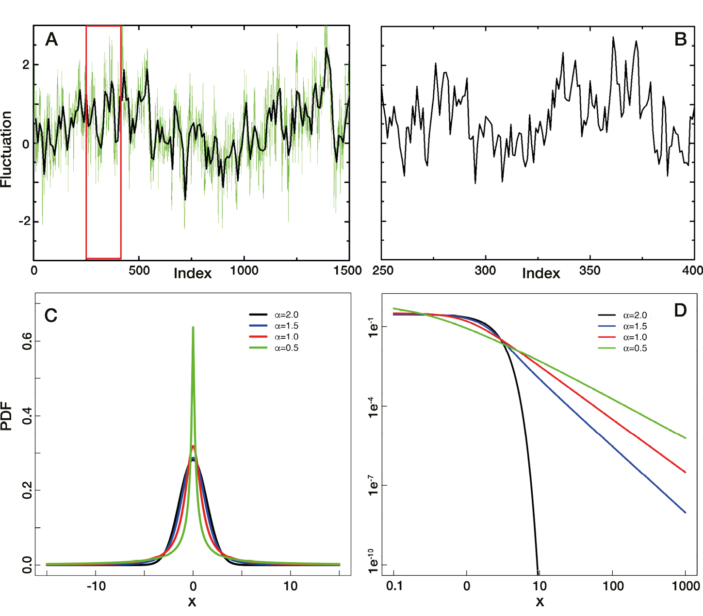
Figure 1: (A-B) Time series with scaling behavior. (A) A time series with scaling behavior and (B) shows the portion in the red box of (A). After zooming in, time series in (B) shows similar pattern as the time series in (A). (C-D) Probability distribution function of an alpha-stable distribution (C) with linear and (D) logarithmic axis scaling. |
Time series which are displaying the Hurst effect have an intriguing property: they remain statistically similar if one zooms in or out (Fig. 1a-b). Scaling is thus related to the notion of fractality (Mandelbrot 1983; Feder 2013), and is mathematically encapsulated by the following equation:
F(n)∝nH (1)
where n denotes the window size over which the amplitude of the fluctuations (F) is computed. The exponent H is then visualized by plotting the logarithm of F(n) against the logarithm of n. When doing so H corresponds to the slope of the corresponding regression line.
We now show that the Hurst effect may emerge from two different effects: (i) existence of correlations between distant points in time and (ii) long-tailed distribution of the amplitudes of the data of interest.
The first effect indicates that even far away points in time are still relatively strongly correlated; in other words, the serial correlation of a time series decays very slowly. Furthermore, for the scaling effects related to the temporal evolution of time series, the above scaling equation (Eq. (1)) indicates that the knowledge of high-frequency variability allows one to predict the low-frequency variability of a time series.
 |
|
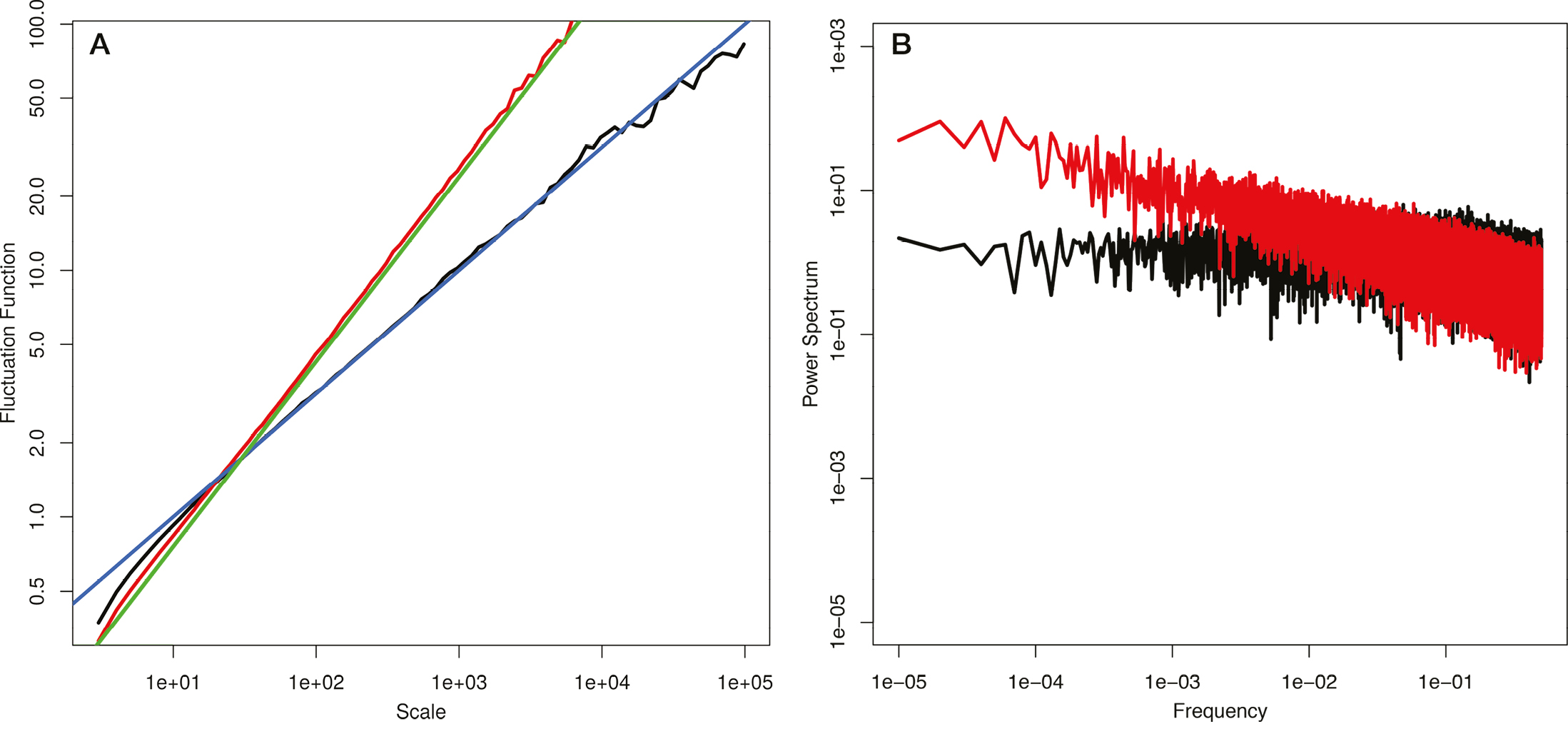
Figure 2: (A) Fluctuation functions for AR(1) process (black line) and scaling model (red line) with regression lines with slopes of 0.5 (blue line) and 0.75 (green line). (B) Power spectrum of AR(1) process (black line) and scaling model (red line). |
To highlight this point we now compare a scaling time series with a short-memory time series in Figure 1 by applying one of the most often used statistical models of climate variability – the auto-regressive process of first order (AR(1)). This is a short-memory process that has a typical auto-correlation timescale. On longer timescales this process acts like independent white noise and the time series values on those timescales become uncorrelated. This is illustrated in Figure 2. There we display a fluctuation analysis of an AR(1) process and a long-memory process. On long timescales the AR(1) process becomes uncorrelated with a slope of 0.5 (compare the fluctuation analysis (black line) with the line with a slope of 0.5 (blue line)). While for the long-memory process (red line), the slope is 0.75 (green line), indicating long-lasting serial correlations. Even very far apart points in time are still correlated, in contrast to a short-memory process.
The contribution related to the probability distribution of the values of a time series is also illustrated in Figure 1. There we display a white noise (uncorrelated values), heavy-tailed distribution (α-stable) in both the typical linear-linear (Fig. 1c) and log-log scalings (Fig. 1d). For α=2 the distribution is the Gaussian distribution with an exponential decay of the probability density function (PDF) while for α<2 it has a power-law decay. The probability for very large events decays more slowly for smaller α values. Hence, extreme events are much more likely to occur for PDFs with a power-law decay of their tails. Heavy-tailed distributions have been shown to be relevant, for instance, for the modeling of the Dansgaard-Oeschger events (Ditlevsen 1999).
Combining the two contributions to the Hurst exponent (i) long memory and (ii) power-law distributed jumps, the Hurst exponent can be written as:
 (2)
(2)
where J denotes the long-memory parameter that determines how fast distant points in time decorrelate, and α is the tail exponent of the PDF (e.g. Franzke et al. 2012). Thus, both effects can contribute to the observed behavior.
What are the implications of scaling?
The long-memory property of many observed climatic time series has consequences for the robust detection of trends. Because long memory leads to the persistence of the time series, long deviations from the mean state are very likely. This can lead to the appearance of apparent trends; so-called stochastic trends (See Fig. 1 of Franzke 2012). Long-memory processes can lead to apparent trends over relative long periods of time even though these trends are not caused by external forcings like increasing greenhouse gas concentrations. These stochastic trends have to be distinguished from deterministic trends which are caused by external forcing.
The presence of long memory in the climate system represents a challenge for the detection of trends in climatic time series. Most trend studies just consider a short-memory process like an AR(1) even though most climate time series also have the long-memory properties (Bunde et al. 2014; Ludescher et al. 2016). This leads to bias in trend detection. In those cases, one is much more likely to assign a trend to be statistically significant even though it is not (Ludescher et al. 2016). Long memory increases the uncertainty of the trend estimates, but on the other hand the true trend could be much larger than under the short-memory assumption.
The long-memory property also induces clustering of extreme events. Long memory leads to long-term quasi-cycles and stochastic trends, i.e. large values are likely followed by large values and vice versa. This tendency also leads to the fact that extremes are likely followed by other extremes and that there will also be long periods when no extremes will occur. This, in turn, leads to the clustering of extreme events in data, which may be used for the development of early warning systems of extreme events.
Long-memory property is also relevant for climate prediction. The stronger the long memory is, the better predictability we may have. Accordingly, using the scaling in climate, it is possible to design climate-prediction models from the perspective of climate memory.
What are the physical mechanisms of scaling?
Since the long-memory property in the climate system is counterintuitive, it is important to identify the underlying mechanisms which cause scaling in the climate system. The superposition of short-memory processes can lead to the emergence of scaling (Granger 1980). This idea is based on the fact that the climate system is composed of many sub-components with different typical timescales (atmosphere, ocean, cryosphere, etc.) and we then observe their superimposed effect in our measurements. Franzke et al. (2015) show that regime behavior due to nonlinear dynamics can also lead to scaling behavior.
acknowledgements
CF was supported by the German Research Foundation (DFG) through the cluster of excellence CliSAP (EXC177) and the collaborative research center TRR181 "Energy Transfers in Atmosphere and Ocean" at the University of Hamburg. NY was supported by the CAS Pioneer Hundred Talents Program.
affiliations
1Meteorological Institute and Center for Earth System Research and Sustainability, University of Hamburg, Germany
2Institute of Atmospheric Physics, Chinese Academy of Sciences, Beijing, China
contact
Christian Franzke: christian.franzke uni-hamburg.de
references
Bunde A et al. (2014) Nat Geosci 7: 246-247
Ditlevsen PD (1999) Geophys Res Lett 26: 1441-1444
Feder J (2013) Fractals. Springer, 284pp
Franzke C (2012) J Clim 25: 4172-4183
Franzke C et al. (2012) Phil Trans R Soc A 370: 1250-1267
Franzke C et al. (2015) Sci Rep 5: 9068
Granger CW (1980) J Econom 14: 227-238
Hurst HE (1951) Trans Amer Soc Civil Eng 116: 770-808
Ludescher J et al. (2016) Clim Dyn 46: 263-271
Mandelbrot BB (1983) The fractal geometry of nature (Vol. 1). WH Freeman, 468 pp