How scaling fluctuation analysis transforms our view of the climate

Shaun Lovejoy
Applied to numerous atmospheric and climate series, Haar fluctuation analysis suggests a taxonomy with four or five scaling regimes that contain most of the atmospheric and climate variability. This includes a new “macroweather” regime in between the weather and climate.
On scales ranging over a factor of a billion in space and over a billion billion in time, the atmosphere is highly variable (from planetary scales down to millimeters, from the age of the planet down to milliseconds). This is usually conceptualized in a "scalebound" framework famously articulated by M. Mitchell (1976) and that focuses on specific phenomena operating over narrow ranges. At first this served to develop simplified mechanisms and models but today, problems are usually solved using full-blown general circulation models (GCMs) and these have wide-range scaling, power law variabilities. By construction, GCMs respect these spatial and temporal scale symmetries.
In the following brief overview, I describe the wide-range scaling view made possible (and necessary) by modern models and paleo-data, and helped by new nonlinear geophysics analysis techniques.
 |
|
Figure 1: The root mean square (RMS) Haar fluctuation showing the various (roughly power law) atmospheric regimes, simplified and adapted from Lovejoy (2015) where the full details of the sources are given. The dashed vertical lines show the rough divisions between regimes; the macroweather-climate transition is different in the pre-industrial epoch. The high-frequency analysis (lower left) from thermistor data taken at McGill at 15Hz was added. The thin curve starting at 2 hours is from a weather station, the next (thick) curve is from the 20th century reanalysis, the next, "S" shaped curve is from the Epica core. Finally, the two far right curves are benthic paleo temperatures (from "stacks"). The quadrillion estimate is for the spectrum, it depends somewhat on the calibration of the stacks. With the calibration in the figure, the typical variation of consecutive 50 million year averages is ±4.5°C (Δt=108 years, RMS ΔT = 9°C). If the calibration is lowered by a factor of ≈3 (to variations of ±1.5°C), then the spectrum would be reduced by a factor of 32. On the other hand, the addition of the 0.017s resolution thermistor data increases the overall spectral range by another factor of 108 for a total spectral range of a factor ≈1023 (for scales from 0.017s to 5x10⁸ years). |
We now know that Mitchell was wrong by a factor of perhaps as much as a quadrillion (see Fig. 1a for details); the great bulk of the variability is in the background spectral continuum (Wunsch 2003) that Mitchell considered to be no more than a series of shallow flat "steps": Gaussian white noises and their integrals.
The continuum can be divided into four or five scaling regimes (Fig. 1) in which mean absolute temperature fluctuations ΔT vary with timescale Δt as ΔT≈ΔtH (for Gaussian processes, there are other equivalent definitions of H, see Franzke and Yuan, this issue). From fast to slow, these regimes alternate in the sign of H from weather, macroweather, climate, macroclimate and megaclimate (this is a proposed taxonomy, the macroclimate regime is very short and may be better considered as a broad quasi-oscillatory regime). When H>0, the temperature "wanders", it appears unstable. When H<0, successive fluctuations tend to cancel, so that as the period Δt is increased, temperature averages converge, they appear to be stable. Such scaling regimes arise whenever the dominant dynamical processes respect a temporal-scale invariance symmetry. An important feature is that scaling processes generally exhibit long-range statistical dependencies implying potentially huge memories that can be used for prediction.
 |
|
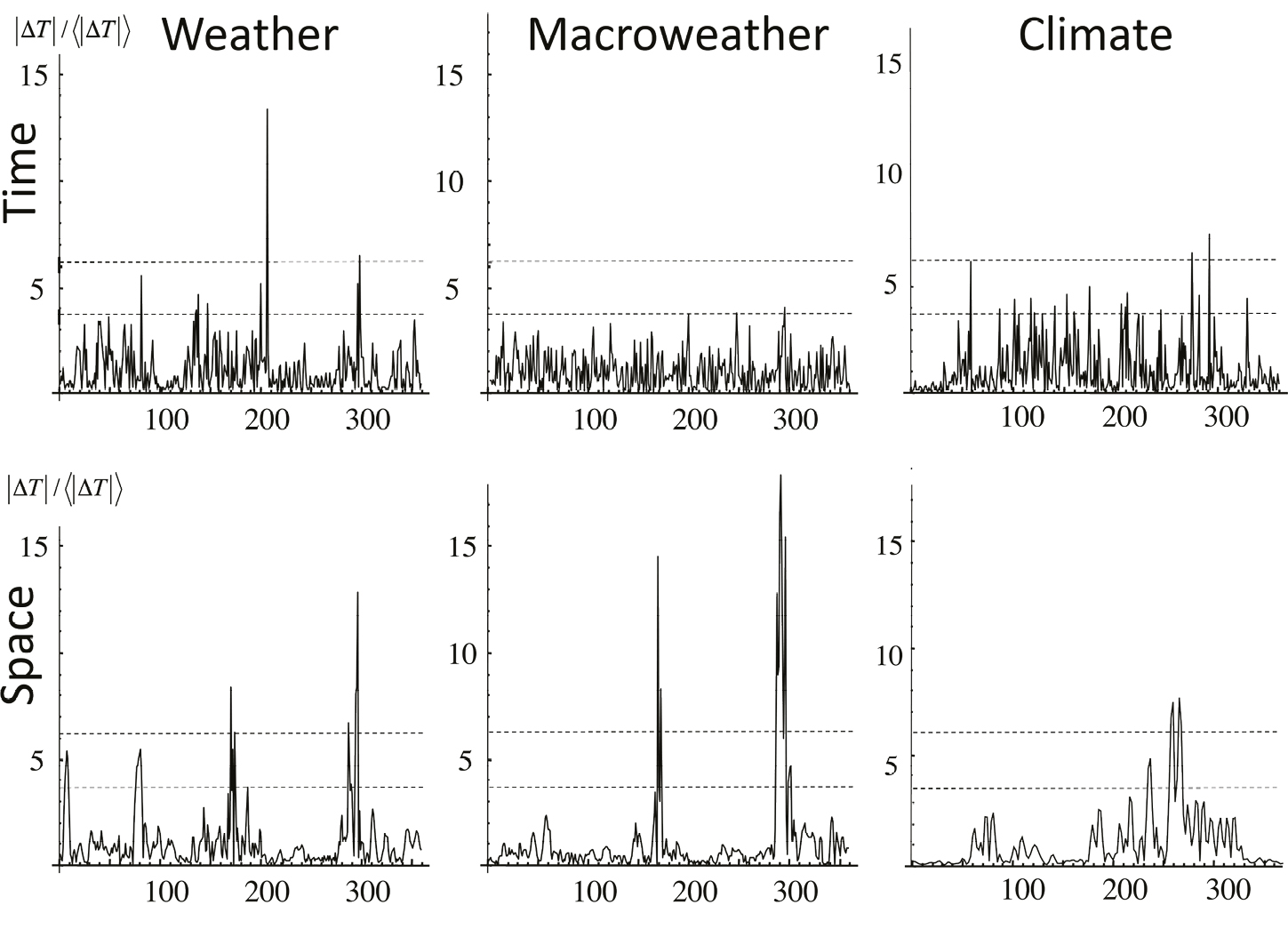
Figure 2: A comparison of the "spikiness" (intermittency) in time (top) and space (bottom), of weather, macroweather and climate series and transects. The graphs have 360 points and show the absolute differences between consecutive values normalized by their means. Each graph has two parallel dashed lines; the lower one corresponds to a Gaussian probability of 1/360, the level of the expected maximum value. The upper dashed line corresponds to a (Gaussian) probability of one in a million. While the spatial intermittencies (bottom) are strong, the temporal intermittencies are nearly absent from the macroweather series (upper middle). Adapted from Lovejoy (in press). Upper left: Hourly temperature data from 1-15 January 2006, from a station in Lander Wyoming. Upper middle: 20C Reanalysis (20CR) from 1891-2011; each point is a four-month average, the data are from a single 2x2° grid point over Montreal, Canada (45°N). Upper right: GRIP (75°N) paleo temperature degraded to 240-year resolution (the present to 86400 years before present, left to right). Lower left: ECMWF reanalysis for the average temperature of 21 January 2000, along the 45°N parallel at resolution of 1° longitude. Lower middle: The same as at left but for the temperature averaged over the month of January 2000. Lower right: The 45°N 20CR temperatures, averaged since 1871. |
This simple scaling picture took a long time to emerge. At first, this was because paleo data were limited and our views were scalebound. Later, it was because analysis techniques were either inadequate (e.g. when fluctuations were quantified via differences or from autocorrelations), or were simply too difficult to interpret (most wavelets and detrended fluctuation analysis), or when using spectral analysis whose interpretations can be very sensitive to "spikiness" (Fig. 2) and has lead to numerous ephemeral, spurious claims of oscillations.
The situation is clarified by the systematic use of simple-to-interpret Haar fluctuations ΔT(Δt). Over the interval from time t to t-Δt, (i.e. at scale Δt), ΔT(Δt) is simply the absolute value of the average of the series T(t) over the first half of the interval (from t-Δt to t-Δt/2) minus the average over the second half (from t-Δt/2 to t). When typical absolute fluctuations decrease with scale (H<0), H quantifies the rate at which anomalies decrease as they are averaged over longer and longer timescales. Conversely, when ΔT(Δt) values increase with scale Δt (H>0), H quantifies the rate at which typical differences increase. Haar fluctuations are useful for processes with -1<H<1 and this encompasses virtually all geoprocesses. Historically, Haar fluctuations were the first wavelets, yet one does not need to know any wavelet formalism to understand or use them. Although the second-order Haar fluctuations (the mean of ΔT(Δt)2) have the same information as the spectrum, the latter was sufficiently difficult to interpret that the "background" was badly misrepresented.
The timescales of the transitions from one regime to another have fundamental interpretations. For example, the inner scale τdis for weather is the dissipation scale and the outer scale is the typical lifetime of planetary structures: τw≈5-10 days, itself determined by the energy rate density (W/kg) due to the solar forcing (Lovejoy and Schertzer 2010). The next regime, "macroweather", is reproduced by weather models (either GCM control runs or the low-frequency behavior of stochastic turbulence-based cascade models). Without external forcings, averages converge to a unique climate so that macroweather continues to arbitrarily large timescales. However, at some point (τc) external forcings and/or slow internal processes become dominant, there is a transition to the climate regime. In the industrial epoch τc≈20 years; in the pre-industrial epoch, τc≈centuries to millennia (Huybers and Curry 2006, see Fig. 1).
A key goal for PAGES’ Climate Variability Across Scales (CVAS) working group is to clarify the spatial (and epoch to epoch) variability and origin of τc: it is not obvious that either solar or volcanic forcings are sufficient to explain it. It seems likely that slow processes including land-ice and/or deep ocean currents may be needed. At Milankovitch scales, H again changes sign and even larger scale (megaclimate) regimes (far right in Fig. 1) has H>0 again.
The scaling has consequences. For example, hiding behind seemingly ordinary signals, there is often strong intermittency; "spikiness". This is visually illustrated in Figure 2 which compares the absolute changes of series (top) and transects (bottom), normalized by their means. Also shown are the expected levels of the maxima for Gaussian processes (bottom dashed lines), and the levels expected at a probability level of one in a million (top dashed lines). One can see that with unique exception of macroweather in time, the signals all hugely spiky. This "intermittency" has two related aspects: extreme jumps (non-Gaussian probabilities) with the jumps themselves clustered hierarchically: clusters within clusters. As anyone familiar with spectral analysis knows, these jumps have large impacts on the spectra; they generate random spectral peaks that can be highly statistically significant when inappropriate – yet standard - Gaussian statistical significance tests are used. In climate applications, they are regularly responsible for ephemeral claims of statistically significant periodicities.
If the process is scaling, then in general the clustering is different for each level of spikiness, requiring a hierarchy of exponents. For example, typical fluctuations near the mean are characterized by the exponent C1 (technically, C1 is the fractal codimension of the typical spike sparseness). Similarly, the probability of an extreme fluctuation ΔT exceeding a threshold s will be a ("fat-tailed"), power law probabilities Pr(ΔT>s) ≈ s-qD for the probability of a random fluctuation ΔT exceeding a fixed threshold s. qD is another exponent; starting with Lovejoy and Schertzer (1986), qD has regularly been estimated as ≈5 (weather and climate temperatures). Depending on the value of qD, extreme fluctuations occur much more frequently than would classically be expected. They are easily so extreme that they would spuriously be considered "outliers". Such events are sometimes called "black swans" (Taleb 2010) and it may be difficult to distinguish these "normal" extremes from tipping points associated with qualitatively different processes, although either might be catastrophic.
A key objective of CVAS is to go beyond time series, to understand variability in both space and space-time. In the weather regime, the spatial H exponents are apparently the same as in time. This is a consequence of the scaling of the wind field and of the existence of a well-defined size-lifetime relationship (Lovejoy and Schertzer 2013). However in macroweather – to a good approximation (verified empirically as well as on GCM and turbulence models) – one has "space-time statistical factorization" so that the joint space-time statistics such as the spectral density satisfies P(em>ω,k)≈P(ω)P(k) and the space-time relationship can be quite different than in weather (Lovejoy and Schertzer 2013). This is important since – without contradicting the existence of teleconnections – it statistically decouples space and time, transforming the GCMs "initial value" problem into a much easier to handle stochastic "past value" (but fractional order) macroweather forecasting problem.
The systematic application of nonlinear geophysics analysis and models-to-climate data has only just begun. CVAS will help take it to the next level.
affiliations
Department of Physics, McGill University, Montreal, Canada
contact
Shaun Lovejoy: lovejoy physics.mcgill.ca
references
Huybers P, Curry W (2006) Nature 441: 329-332
Lovejoy S (2015) Clim Dyn 44: 3187-3210
Lovejoy S (in press) Weather, Macroweather and Climate: big and small, fast and slow, our random yet predictable atmosphere, Oxford U. Press, 250 pp
Lovejoy S, Schertzer D (1986) Ann Geophys 4B: 401-410
Lovejoy S, Schertzer D (2010) Atmos Res 96: 1-52
Mitchell JM (1976) Quat Res 6: 481-493
Taleb NN (2010) The Black Swan: The Impact of the Highly Improbable, Random House, 437 pp