Scaling of global temperatures explained by linear energy balance models

Kristoffer Rypdal and Hege-Beate Fredriksen
Scale invariance of natural variability of global surface temperatures is often interpreted as a signature of nonlinear dynamics. However, the observed scaling can be adequately explained by linear energy balance involving subsystems with different response times.
The analysis of instrumental data and proxy reconstructions of global mean surface temperature (GMST) reveals higher variability on longer timescales than expected, provided we assume that the surface temperature responds as if it were a body with a heat capacity corresponding to the mass of the ocean mixed layer. The power-spectral density of the temperature variability of such a body, driven by the stochastic forcing from atmospheric weather systems, should have the shape of a Lorentzian distribution; a flat spectrum for low frequencies f, and a power-law spectrum P(f)~f-2 for high frequencies. The transition between the two regimes would be at a transition frequency fT=(2πτ)-1, where τ is the exponential decay time (the time constant) for a perturbation of the equilibrium temperature. The stochastic process that exhibits such a spectrum is sometimes referred to as red noise. The actual observed spectrum tends to follow the power-law P(f) ~f-1, which is called pink noise or 1/f-noise. This power-law scaling has been demonstrated for Holocene climate in a large number of papers, and Rypdal and Rypdal (2016a) also found such a spectrum for the background noise in δ18O of Greenland ice-core records during the last glaciation by eliminating the sudden transitions between warm and cold periods that have been found in ice-core data at that time. Thus, the observed power-law scaling does not comply with the Lorentzian spectra of simple linear energy balance models (EBMs), and a popular explanation has been nonlinearity in the response. Nonlinearity, however, offers no real explanation of the scaling of the background GMST variability until a nonlinear theory of the GMST spectrum is in place, and at present it is not. Our objective in this article is to show that a linear EBM may explain the observed spectrum, provided some plausible additional physics is added. For this purpose, we need to give a brief description of how such models work.
Energy balance models and their linearization
 |
|
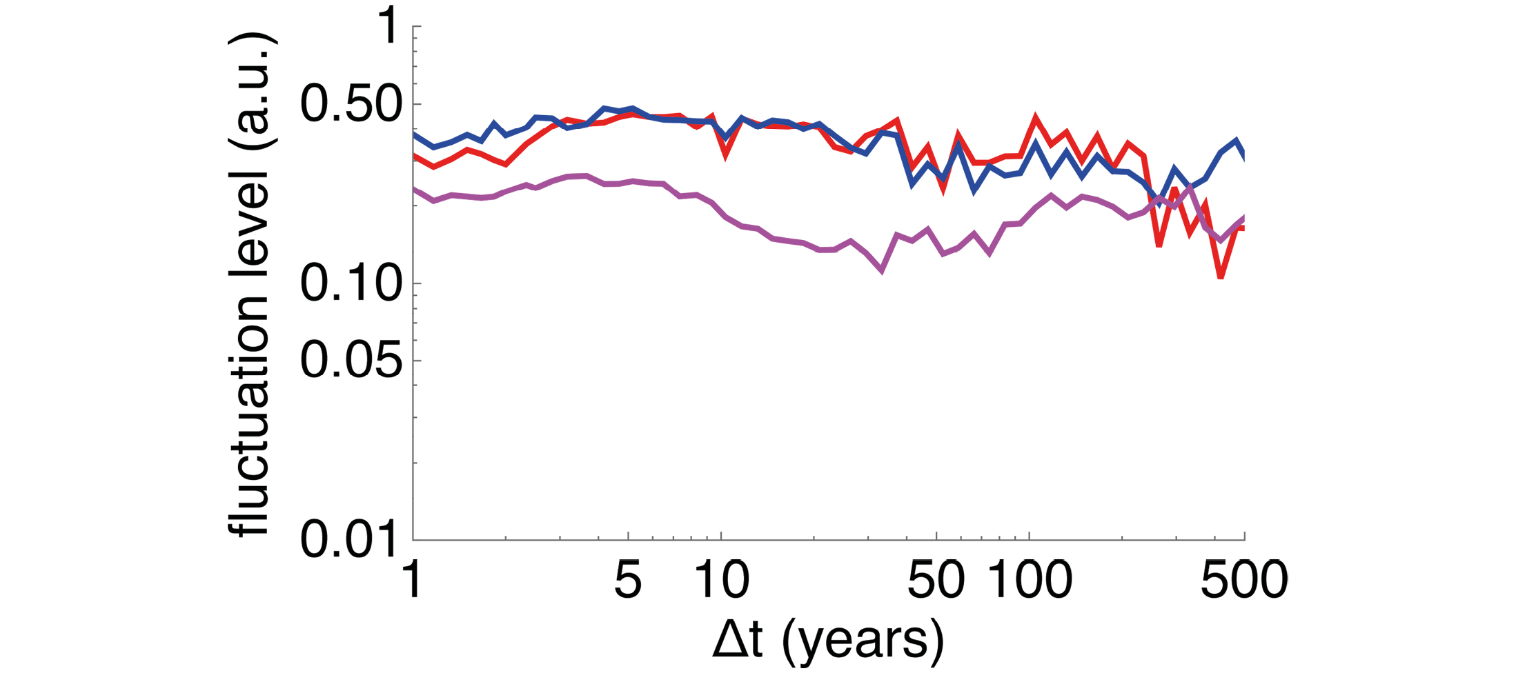
Figure 1: Fluctuation levels of GMST (in arbitrary units) obtained in the NorESM model as a function of timescale ∆t. Red: Fluctuation level of GMST response to the sum of volcanic and solar forcing. Blue: The same for sum of responses to volcanic and solar forcing. The overlap of the curves suggests linearity of the response. Magenta: The same for control run, reflecting fluctuation level of internal variability. |
First it should be mentioned that EBMs of the GMST often contain nonlinearity in the form of a temperature dependence of the surface albedo due to the snow and ice cover. Such models exhibit multiple fixed points, bifurcations with sudden transitions, and hysteresis. An excellent review of such models was given by North et al. (1981), where also the description of internal variability in the global temperature is introduced through stochastic forcing terms. For a climate system far from tipping points, however, the traditional EBMs exhibit a stable fixed point, and for moderate perturbations of this energetic equilibrium the equations of energy balance can be linearized. This linearization of the GMST response is supported by general circulation models (GCMs). Linearity of the temperature response in GCMs has been extensively studied over the last two decades, and the majority of studies find only weak nonlinearities in the global response. For instance, Rypdal and Rypdal (2016b) demonstrated, by analyzing millennium-long data sets from the Norwegian Earth System Model (NorESM), that linearity of the response prevails (Fig. 1).
The one-box model and the exponential response to forcing
An exponentially decaying response function derives naturally from the simplest conceivable model of the GMST response to forcing; the zero-dimensional, linear energy balance equation; C dT/dt=F-λT. Here T is the surface temperature anomaly and F is the perturbation of radiation flux density (the forcing) giving rise to T. In general, the forcing has a deterministic and a stochastic component, the latter representing the influence of the chaotic variability of atmospheric weather systems. CT is the change in heat content per square meter in a vertical column when GMST changes by T, hence C represents the effective heat capacity per unit area of this system, which is dominated by the heat capacity per unit area of the upper few hundred meters of the oceans. The model neglects the heat exchange between this layer and the deep ocean, and in this respect, it is based on the same assumptions as aqua-planet GCMs. The term –λT represents the change of flux density of top of atmosphere longwave outgoing radiation in response to the temperature change T, and is corrected for fast feedback processes. If F results from an abrupt change of forcing, then T will eventually relax to a new equilibrium state T=SF, where the parameter S=λ-1 is the equilibrium climate sensitivity. The time evolution of the relaxation can be written as T(t)=FS[(1-exp (-t/τ)], with time constant τ=CS. By Fourier transforming the one-box model we obtain the Lorentzian spectrum,
 (1)
(1)
where T̃(f) and F ̃(f) are Fourier transforms of T(t) and F(t), respectively. From this relation, one observes that the response on timescales longer than the time constant τ is simply obtained by multiplying the forcing by the sensitivity S, while the response on fast timescales (f>f_T) is weaker due to the thermal inertia. If the forcing grows rapidly, the temperature, and hence the radiation-loss term –λT, will grow more slowly and the climate system will accumulate heat until a new thermal equilibrium is attained. This delayed warming is what is referred to as “the warming in the pipeline”.
Multi-box models and the power-law response
 |
|
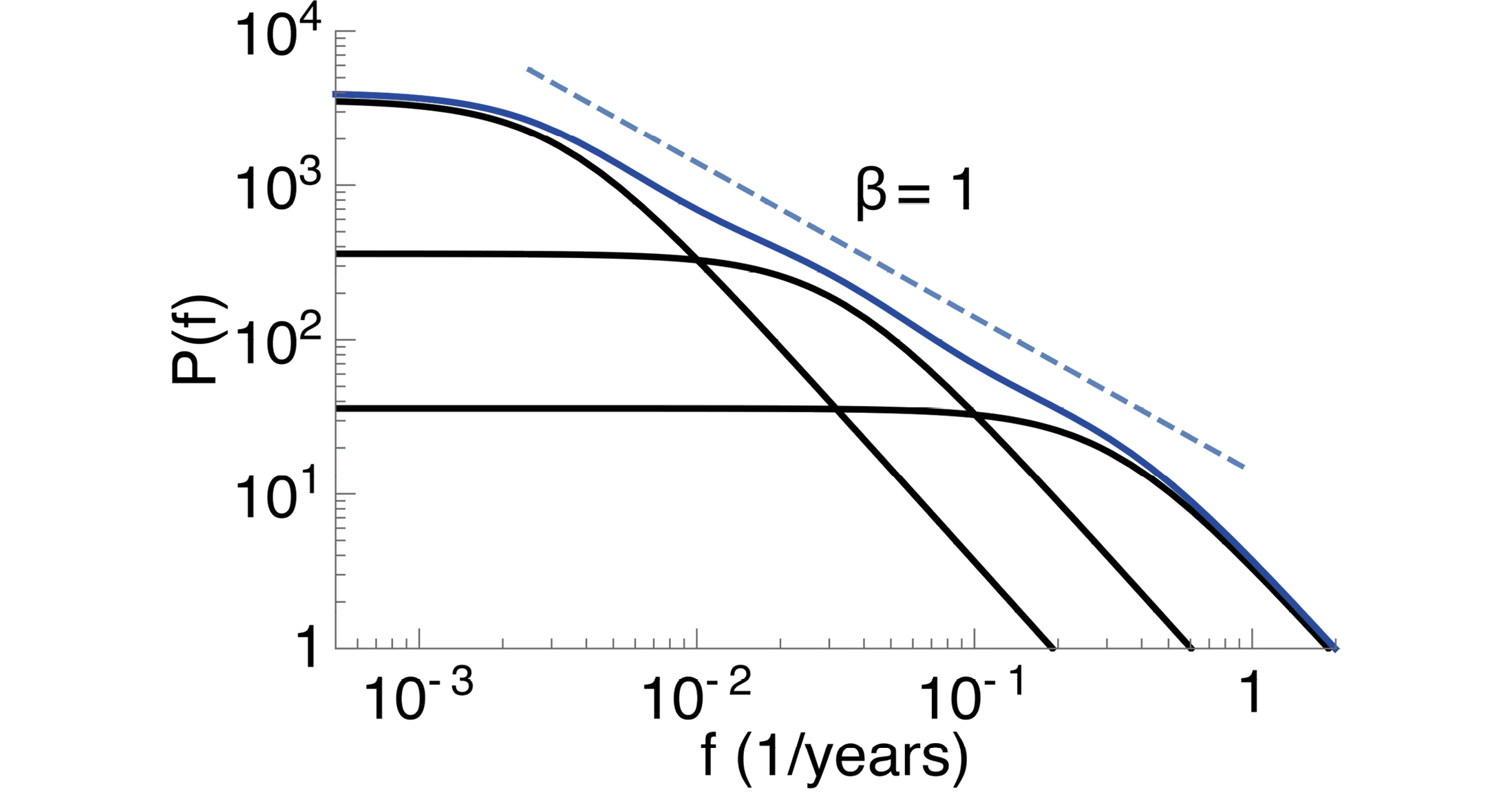
Figure 2: Temperature fluctuations described by a multi-box model can be written as a sum of the outputs from the one-box model with different response times. Here we use τ1=0.5, τ2=5 and τ3=50 years, and each black curve shows the spectra as given by Eq. (1). The sum of these is the blue curve, well approximated by the power law P(f)~f-1 (dashed line). |
It has been known for several decades that atmospheric-ocean GCMs exhibit climate responses on separated timescales, i.e. there is more than one time constant involved in the response. A simple two-box generalization of the one-box model allows for heat exchange between the upper mixed layer of the ocean and the deep ocean, and the general response to a forcing starting at time t = 0 can be written as a convolution integral T(t)=∫t0 G(t-t') F(t') dt', where the response kernel is a superposition of two decaying exponential functions with different e-folding times τ1 and τ2. Geoffroy et al. (2013) estimated the parameters of a linear two-box energy balance model by data from runs of a large number of GCMs with step-function forcing and linearly increasing forcing, respectively. They found a very good fit to the simulated global temperature. Rypdal and Rypdal (2014) demonstrated that an excellent fit to global instrumental temperatures and Northern hemisphere temperature reconstructions over the last two millennia could be obtained by replacing the superposition of exponentials by a power-law function G(t)~tβ/2-1 with β≈1. If F(t) is assumed to be a white noise representing the stochastic forcing, the resulting internal GMST-variability exhibits a spectrum P(f)~f-β similar to the observed one. Fredriksen and Rypdal (2017) showed that there is a correspondence between this power-law scaling and the spectra obtained from the linear box models by developing a formalism of N boxes exchanging heat with each other (Fig. 2). In fact, they obtained spectra reminiscent to those obtained from observations and GCMs by restricting the model to three boxes, suggesting that scaling observed in GMST is a result of linear energy exchange in a system with multiple response times.
affiliations
Department of Mathematics and Statistics, UiT The Arctic University of Norway, Tromsø, Norway
contact
Kristoffer Rypdal: kristoffer.rypdal uit.no
references
Fredriksen H-B, Rypdal M (2017) J Clim 30: 7157-7168
Geoffroy O et al. (2013) J Clim 26: 1841-1857
North GR et al. (1981) Rev Geophys Space Phys 19: 91-121
Rypdal M, Rypdal K (2014) J Clim 27: 5240-5258