Inferring past climate variations from proxies: Separating climate and non-climate variability

Thomas Laepple1, T. Münch1,2 and A.M. Dolman1
The statistical properties of climate variability are often reconstructed and interpreted from single proxy records. However, variation in the proxy record is influenced by both climate and non-climate factors, and these must be understood for climate inferences to be reliable.
Before interpreting the temporal variability in any climate proxy record we first need to study the reproducibility of the measured signal. One way of doing this is to compare variations in nearby records that were subject to the same history of the target climate variable, such as local temperatures. In simple terms, features that appear only in individual records most likely represent non-climate variability, whereas those that reproduce across multiple proxy records potentially represent variations in climate. Such a comparison provides an upper limit on the climate information contained in the record.
Reproducibility is a necessary but not sufficient condition for a reconstructed signal to be inferred as climatic in origin. Spatially coherent variability can also be caused by environmental changes independent of the variable of interest. For example, changes in ocean circulation might cause large-scale changes in water masses that affect the preservation of marine climate proxies and thus the recorded signals. One way to overcome this is to compare the record to independent estimates of variations in the target variable; either from instrumental records such as weather stations, or from independent climate proxies that record the same target variable. Performing such comparisons in the frequency domain allows for a more detailed characterization of the proxy system: in particular, it highlights the timescales at which the signal is preserved rather than obscured by noise and where it might be reliably interpreted as climate.
The procedure outlined above is idealized, and may in many cases be unrealistic due to limitations in resources such as cost, manpower, or replicate proxy material. However, advances in the collection, processing and analysis of the proxy material now make it often feasible to obtain the volume of data required to carry out such analyses.
Oxygen isotope records on the Antarctic Plateau
Here we give an example of the first steps of this approach for the isotopic composition of water archived in firn and ice at the drilling site of the EPICA Dronning Maud Land ice core (EDML) at Kohnen Station on the Antarctic Plateau.
Isotopic variations in ice are usually interpreted as a proxy for local air temperature at the location of snowfall. However, in reality, many processes influence the signal, starting with the evaporation source of water and including depositional and post-depositional effects (Casado et al. this issue). Indeed, previous studies have shown that the reproducibility of isotope profiles is poor on monthly to multi-decadal timescales for low-accumulation sites such as EDML (< 100 mm w.e. a-1; Karlöf et al. 2006). Thus, when interpreting isotope records it is essential to quantify the proportion of variability which is related to the target variable versus that of the other sources.
Spatial and vertical isotope variability
 |
|
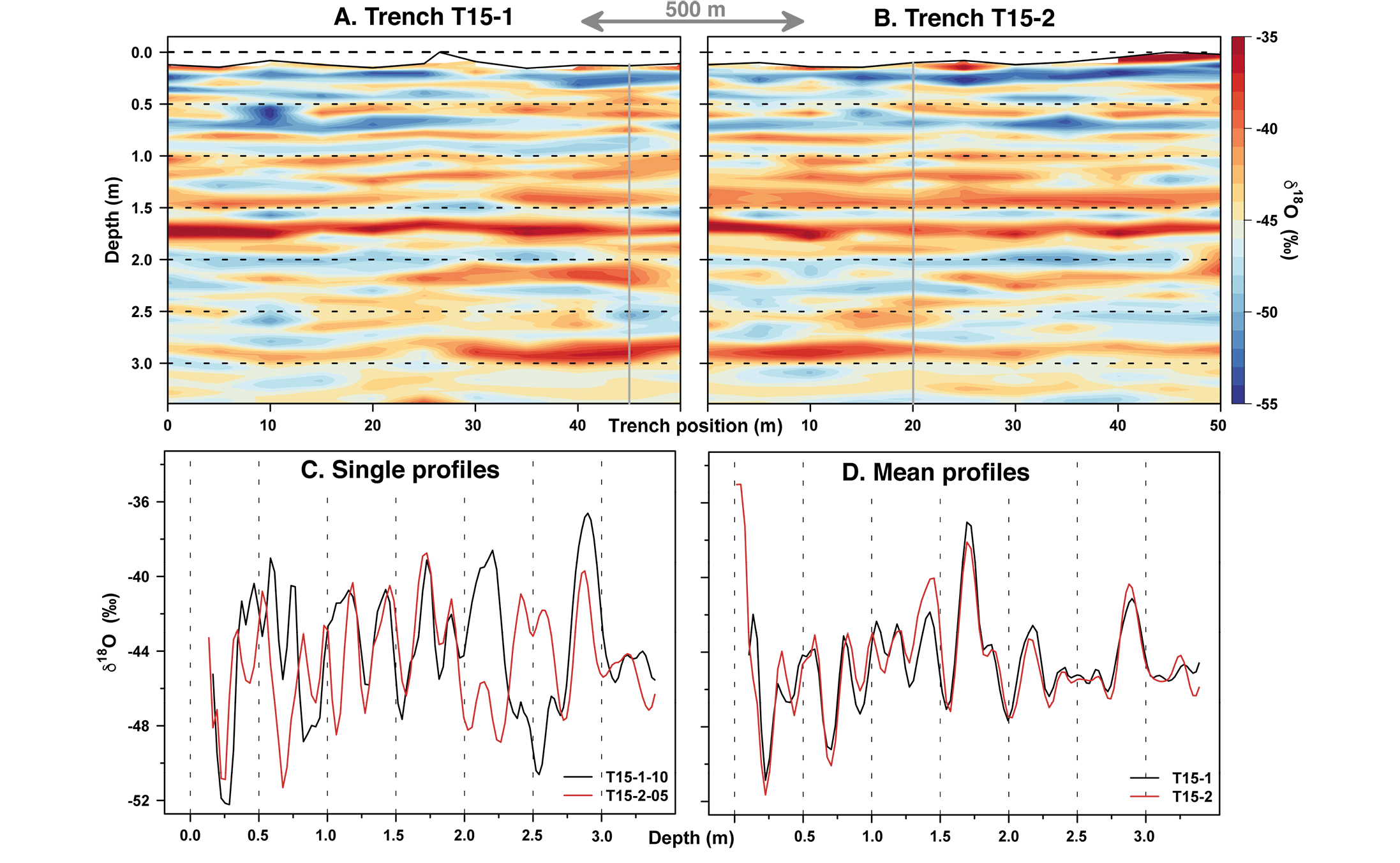
Figure 1: The oxygen isotope records of the snow trenches T15–1 and T15–2 from the EDML site. Panels (A) and (B) show the isotope variations in each trench as two-dimensional color images; panel (C) the comparison of two selected individual isotope profiles (the positions marked as vertical lines in (A) and (B)); and panel (D) the comparison of the mean profiles obtained by averaging across the individual profiles of each trench. Figure modified from Münch et al. 2017. |
We extended the concept of replicate coring by analyzing the horizontal and vertical variations of snow density and isotopic composition at EDML in several 50 m long and 1–3 m deep snow trenches. Isotope and density profiles were sampled at 0.2 to 5 m intervals along the wall of each trench which allowed us to create two-dimensional images that characterize the proxy variations from the centimeter to the hundred-meter scale (Laepple et al. 2016; Münch et al. 2016, 2017; Fig. 1).
Looking at the isotopic composition, we found visible layers that indicate a representative signal but also show significant horizontal variability (Fig. 1A, B). Consequently, the mean correlation (r) between any two individual vertical profiles separated by more than 10 m (equivalent to comparing two normal firn cores) was just 0.5, but between the two trench-averaged vertical profiles the correlation was much higher (0.9; Fig. 1D). We could explain the observed spatial variability by a simple model describing the local stratigraphic noise as a process with a horizontal decorrelation length of ~1.5 m (Münch et al. 2016). This model provides an upper bound on the reliability of seasonal to interannual-timescale climate reconstructions from single firn cores for our study site. It further shows that averaging several vertical profiles, separated by distances greater than the decorrelation length, will reduce the noise and produce a signal that is representative over a scale of at least 500 m (Fig. 1D). Similar studies are needed and are ongoing at other sites to create a mechanistic model of the stratigraphic noise, or to parameterize the noise as a function of the depositional parameters (Fisher et al. 1985).
The power spectra of proxy versus climate
 |
|
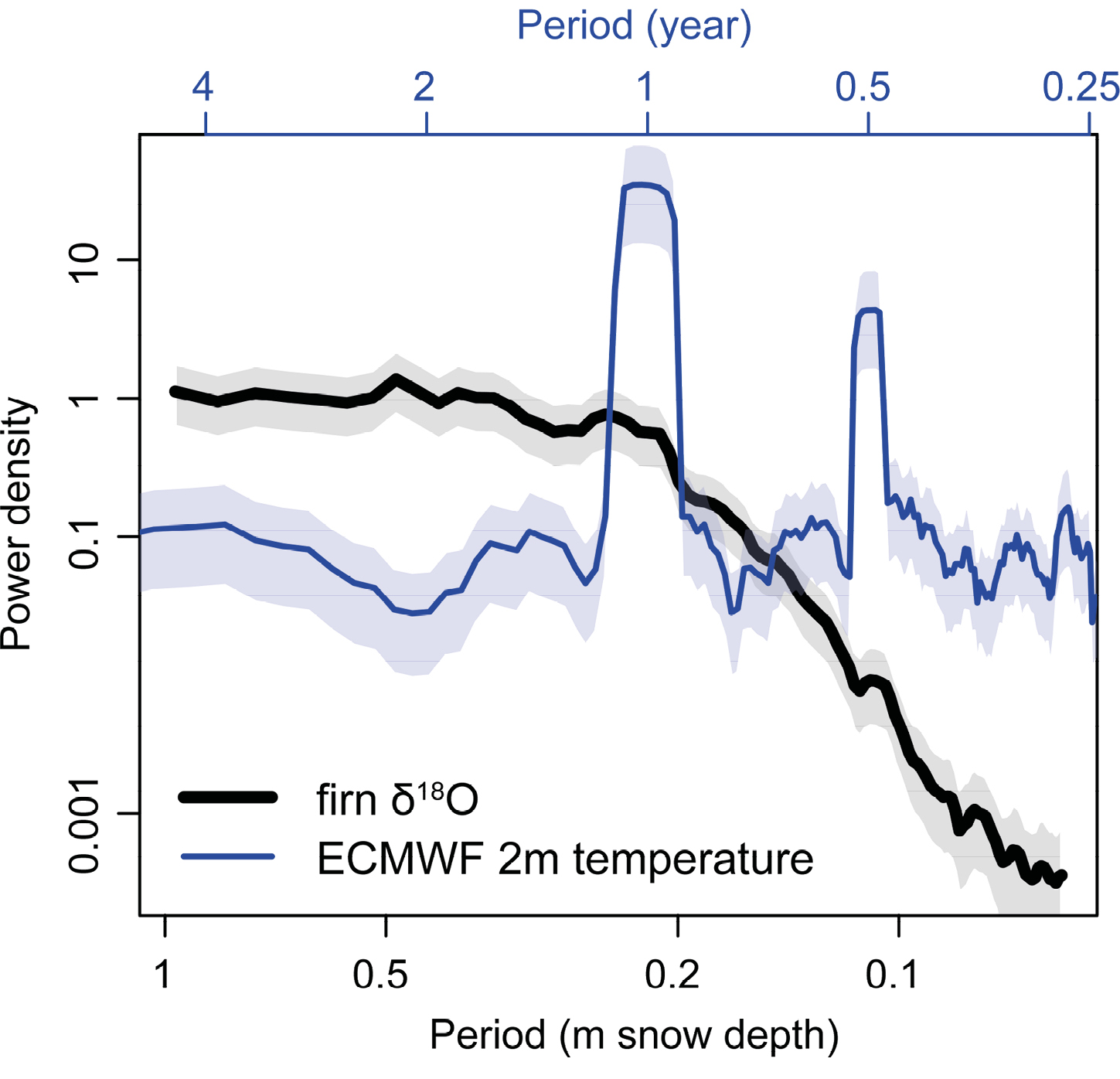
Figure 2: Power spectra of the δ18O variations from the snow trench data (average spectrum across 22 3.4 m deep trench profiles, black) and of the monthly 2 m air temperatures (1979-2016) from the European Centre for Medium-Range Weather Forecasts (ECMWF) reanalysis (blue) at EDML. The horizontal and vertical scales are aligned assuming an accumulation rate of 22 cm snow per year and using the modern spatial δ18O to temperature relationship of 0.8 ‰ K-1, respectively. For details on the spectral analyses see Laepple et al. 2017. |
At EDML, the dominating surface temperature signal is the annual cycle: its first two harmonics explain 95% of the monthly variance in the last 40 years (ERA interim reanalysis, Dee et al. 2011). Comparing the power spectra of the instrumentally observed temperature signal with that recorded by the oxygen isotopes in the trenches shows the fundamental difference between the records (Fig. 2). On scales shorter than annual (less than ~0.2 m snow thickness), the oxygen isotopes show less variability than the temperatures. This is expected since firn diffusion dampens small-scale isotopic variability (Johnsen et al. 2000). In contrast, for interannual variations (greater than ~0.3 m snow thickness), the isotopic variability is around one order of magnitude higher than that of temperature. Also of note is that the annual cycle and its harmonics are largely missing in the isotope record. Both findings can be explained by precipitation intermittency (Persson et al. 2011), interannual variations in snow accumulation and snow redistribution which corrupt and alias the seasonal cycle, shifting its power to lower frequencies (Laepple et al. 2017). One should therefore avoid a direct interpretation of the spectrum of variability in isotope records in terms of temperature signals.
Outlook and implications for other proxies
Using the example of oxygen isotopes of water at the EDML site, our analysis demonstrates the need to consider the reproducibility of proxy records. Since the analysis was restricted to the top 3.5 m of firn, it applies to seasonal and interannual-scale variations. To determine the implications for centennial to millennial-scale climate reconstructions, the temporal correlation structure of the noise has to be known at those scales, therefore we are currently extending our analysis to deeper firn and ice cores. A simple comparison with the local instrumental temperature record demonstrated the fundamentally different nature of the isotope and temperature signals on seasonal to interannual timescales. While the deviations are not unexpected given our knowledge of precipitation intermittency, redistribution and firn diffusion, they caution against a simplistic interpretation of the spectrum of variability in proxy records. Similar studies for other archives, such as sediment cores, would be useful and would assist and improve the interpretation of climate variability derived from proxies (Laepple and Huybers 2013). In addition, they would provide a much-needed test bed for proxy system models that take a mechanistic approach to the same problem (Dee et al. 2015).
affiliations
1Alfred Wegener Institute Helmholtz Centre for Polar and Marine Research, Potsdam, Germany
2Institute of Physics and Astronomy, University of Potsdam, Germany
contact
Thomas Laepple: tlaepple awi.de
references
Casado M et al. (2017) PAGES Mag 25(3): 146-147
Dee DP et al. (2011) Q J Royal Meteorol Soc 137: 553-597
Dee S et al. (2015) J Adv Model Earth Syst 7: 1220-1247
Fisher DA et al. (1985) Ann Glaciol 7: 76-83
Johnsen SJ et al. (2000) Phys Ice Core Rec: 121-140
Karlöf L et al. (2006) J Geophys Res 111: F04001
Laepple T, Huybers P (2013) Earth Planet Sci Lett 375: 418-429
Laepple T et al. (2016) J Geophys Res Earth Surf 121: 1849-1860
Laepple T et al. (2017) Cryosphere Discuss: 199
Münch T et al. (2016) Clim Past 12: 1565-1581