Modeling the climate of the Last Glacial Maximum from PMIP1 to PMIP4

Kageyama M, Abe-Ouchi A, Obase T, Ramstein G and Valdes PJ

> Access contents of this issue

> Download this article as pdf

Past Global Changes Magazine

29(2)

80-81

2021

https://doi.org/10.22498/pages.29.2.80

Masa Kageyama¹, A. Abe-Ouchi², T. Obase², G. Ramstein¹ and P.J. Valdes³

The Last Glacial Maximum is an example of an extreme climate, and has thus been a target for climate models for many years. This period is important for evaluating the models' ability to simulate changes in polar amplification, land–sea temperature contrast, and climate sensitivity.

The Last Glacial Maximum (LGM, ∼21,000 years ago), a period during which the global ice volume was at a maximum and global eustatic sea level at a minimum, inspired some of the first simulations of past atmospheric circulation and climates (Gates 1976; Manabe and Broccoli 1985a; Manabe and Broccoli 1985b; Kutzbach and Wright 1985). Because of the extreme conditions during this period, the LGM was documented quite early, notably through the CLIMAP project (e.g. CLIMAP Project Members 1981). This early work gave rise to many questions: how cold, how dry, how dusty was it, and why? How was the Northern Hemisphere ice sheet sustained? How did the massive ice sheet impact the atmospheric and oceanic circulation? What were the impacts of these ice sheets on climate, compared to the impact of other changes in forcings and boundary conditions, such as the decrease in greenhouse gas concentrations? What climate feedbacks were induced by vegetation, the cryosphere, dust, and permafrost? Are the features from paleodata reconstructions also found in the results of the models that are routinely used to compute present and future climate changes? Climate reconstructions for the LGM were also hotly debated, sometimes in relation to one another, such as for tropical cooling over sea and over land (e.g. Rind and Peteet 1985).

In the beginning

PMIP was launched as a result of a NATO Advanced Research Workshop in Saclay, France, in 1991 (Joussaume and Taylor, this issue). At that time, several LGM simulations had already been carried out, and the different modeling groups involved in running these experiments had therefore already gathered some experience. However, these simulations were not strictly comparable since they did not use the same forcings or boundary conditions. For example, the CO₂ forcing, which became a central point of LGM climate analyses due to its connection with climate sensitivity, was actually not taken into account in climate simulations until the work of Manabe and Broccoli (1985b), who cited the CO₂ retrieved from Greenland and Antarctic ice cores published by Neftel et al. (1982). At the Saclay meeting, it was clear that many groups of modelers and data scientists were motivated to build a common project to better understand the climate during the mid-Holocene and the Last Glacial Maximum, based on numerical simulations and on syntheses of paleoclimatic reconstructions.

Developing the approach

It took time, intensive debates, and several PMIP meetings to agree on a common approach, forcings and boundary conditions; develop a strategy for paleodata compilations; and establish a methodology for model–data comparison. Therefore, the real launch of the PMIP1 LGM simulations was in 1994. Despite having chosen to adopt an approach that would be as simple as possible, it took no fewer than four newsletters to describe the corresponding experimental protocol (pmip1.lsce.ipsl.fr/ > Newletters). To engage as many groups as possible in this new adventure, the decision was made to allow for two types of simulations to be run for the LGM: one using atmosphere-only general circulation models (AGCMs) and therefore prescribing surface conditions (sea surface temperatures and sea ice from the CLIMAP (1981) reconstructions), the other using AGCMs coupled to slab ocean models, which computed the ocean conditions under the (strong) assumption that the ocean heat transport was similar to the pre-industrial one.

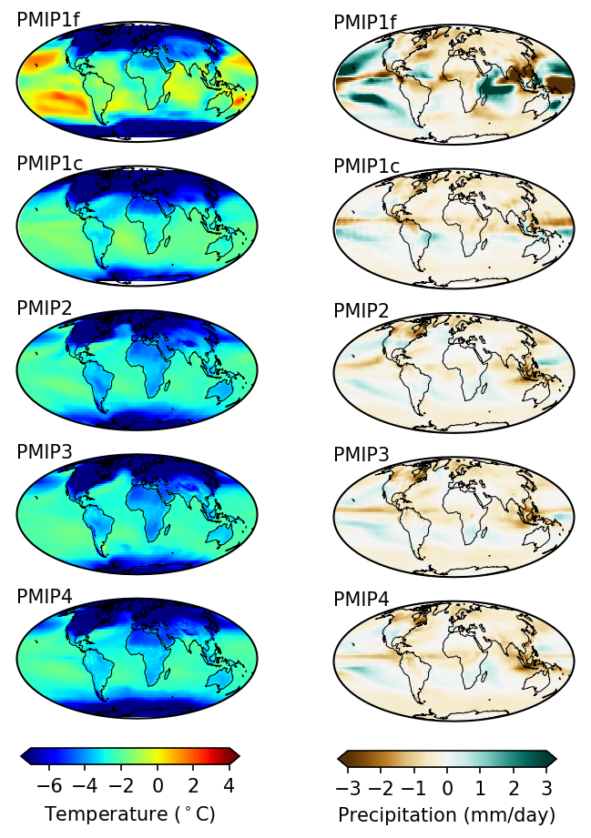
Figure 1: LGM – PI multi-model average anomalies simulated by climate models of the different PMIP phases for Mean Annual Temperature (left) and precipitation (right). PMIP1f: PMIP1-prescribed SST AGCM simulations; PMIP1c: simulations run with AGCMs coupled to slab ocean models. All other PMIP phases used coupled atmosphere-ocean GCMs.

The recommended ice-sheet reconstruction (ICE-4G; Peltier 1994) was the same for both types of experiments. Encouraging groups to run prescribed and computed SST experiments proved to be a wise decision, as this resulted in a total of eight simulations of each type being made available with contrasting results (Fig. 1). The largest difference between the groups of PMIP simulations is clearly between the prescribed SST simulations (labelled "PMIP1f") and the computed SST simulations (labelled "PMIP1c"). Both ensemble means show global cooling, amplified from the equator to the poles, with stronger cooling over the continents than over the oceans. These two large-scale characteristics (later termed "polar amplification" and "land–sea contrast") would be analyzed in all phases of PMIP, as these features are also seen in projections of future climate and should therefore be evaluated. Another topic of analysis was the atmospheric circulation in the vicinity of the large Northern Hemisphere ice sheets, following the striking "split-jet" response found in the pioneer, pre-PMIP simulations. This feature was not systematically found in the PMIP1 experiments, but the response of the atmospheric circulation and its interaction with the oceans remains a topic of active research.

What Figure 1 does not show is that the range of the PMIP1c results was much larger than that for PMIP1f, foreshadowing the need for coupled ocean-atmosphere models (cf. Braconnot et al. this issue). The advent of coupled ocean-atmosphere general circulation models resulted in the launch of the second phase of PMIP in 2002 (Harrison et al. 2002) with an updated ice-sheet boundary condition: ICE-5G (Peltier 2004; Fig. 2). Running these experiments was technically challenging, and it remains so because it forces the climate models out of their "comfort zone" (i.e. the conditions for which the models were initially developed). It requires a long equilibration time, which is very computationally expensive for the latest generation of models. Despite these challenges, the use of these coupled models proved to be very worthwhile, as they allowed for the use of marine data for evaluation, rather than for prescribing boundary conditions. This represented a huge release of the constraints on ocean reconstructions, which did not need to cover all the world's oceans for winter and summer. New ways to compare models and marine data became available, taking into account the indicators' specificities, some of which are still being investigated today. These should help us understand why reconstructions from different indicators sometimes differ significantly (Jonkers et al. this issue).

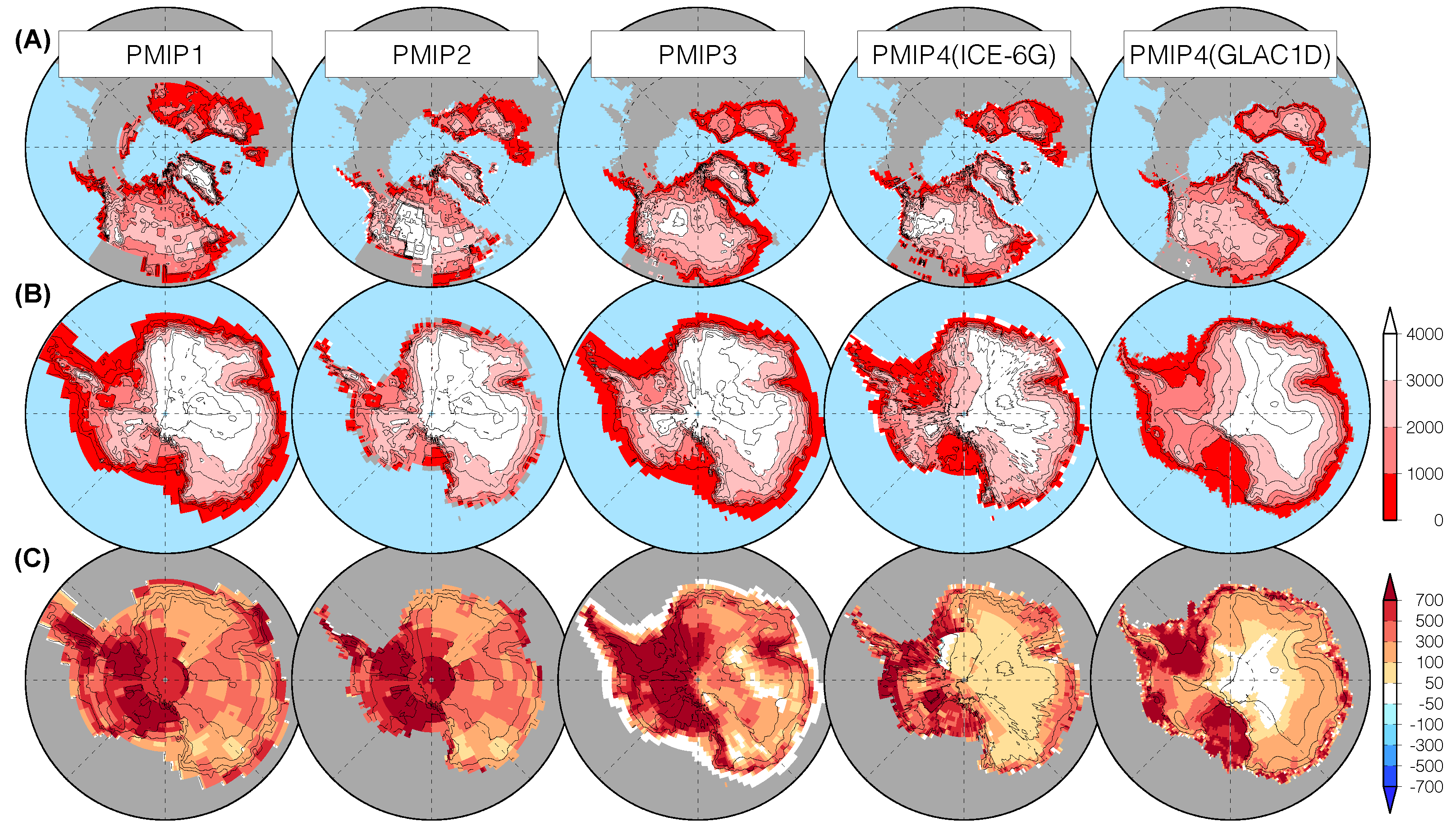
Figure 2: Evolution of the ice sheets used as boundary condition in the different PMIP phases. From the left to right: PMIP1 (ICE-4G; Peltier 1994), PMIP2 (ICE-5G; Peltier 2004), PMIP3 (Abe-Ouchi et al. 2005), PMIP4 (ICE-6G_C; Argus et al. 2014; Peltier et al. 2015), and PMIP4 (GLAC-1D; Ivanovic et al. 2016). (A) The altitude of Northern Hemisphere ice sheets at the LGM; (B) the altitude of Antarctica ice sheet at the LGM; (C) the altitude difference (LGM minus present day).

Progress in PMIP3 and PMIP4

Simulations during the third and fourth phases of PMIP were also run with coupled models, sometimes even with interactive vegetation, dust (see Lambert et al. this issue), and/or a carbon cycle (see Boutttes et al. this issue). While PMIP2 often used lower resolution models compared to those used for future climate projections, the novelty from PMIP3 onwards was that exactly the same model versions were used for both exercises, hence allowing for rigorous comparisons of processes involved in past and future climate changes. Boundary conditions, in particular in terms of ice-sheet reconstructions, were updated for each phase (Fig. 2). Ice-sheet reconstructions for the LGM were a hotly debated topic, but during the first three phases of PMIP, a single reconstruction was chosen. For PMIP3, this reconstruction was derived from three different reconstructions (Abe-Ouchi et al. 2015; Fig 2). Choosing a single protocol was deemed important for all the simulations to be comparable. For PMIP4, however, evaluating the uncertainty in model results related to the chosen boundary conditions was deemed necessary because differences between the ice-sheet reconstructions remained quite large in terms of ice-sheet altitude (Ivanovic et al. 2016; Kageyama et al. 2017). The PMIP4 dataset should ultimately help us reach this goal (most simulations presently available use Peltier's ICE-6G_C reconstruction; Argus et al. 2014; Peltier et al. 2015).

Providing an exhaustive list of the analyses based on these simulations would require more space than is available here. Recurring topics across the four phases of PMIP encompass large-scale to global features, such as climate sensitivity; polar amplification and land–sea contrast; atmosphere and oceanic circulation, in particular the Atlantic Meridional Overturning Circulation; the comparison of model results with reconstructions for various regions; and impacts on the ecosystems. An intriguing feature is that from PMIP2 to PMIP4, even though both models and experimental protocol have evolved, the range of model results (cf. Braconnot et al. this issue regarding the multi-model results in terms of cooling over tropical land and oceans) is quite stable, and within the range reconstructed from marine and terrestrial data. This might sound satisfactory, but in fact is a call for the reduction in the uncertainty of the reconstructions, the reconciliation of reconstructions from different climate indicators, or a better understanding of the differences and a refinement of the methodology regarding model–data comparisons. This would allow us to draw many more conclusions about the LGM in terms of understanding the climate system's sensitivity to changing forcings, and in terms of impacts of climate changes on the environments.

affiliations

¹Laboratoire des Sciences du Climat et de l'Environnement, LSCE/IPSL, UMR CEA-CNRS-UVSQ, Université Paris-Saclay, Gif sur Yvette, France
²Atmosphere and Ocean Research Institute, The University of Tokyo, Japan
³School of Geographical Sciences, University of Bristol, UK

contact

Masa Kageyama: Masa.Kageyamalsce.ipsl.fr

references

Abe-Ouchi A et al. (2015) Geophys Model Dev 8: 3621-3637
Argus DF et al. (2014) Geophys J Int 198: 537-563
Peltier WR et al. (2015) J Geophys Res Solid Earth 120: 450-487
CLIMAP Project Members (1981) Seasonal reconstruction of the Earth's surface at the last glacial maximum. Geol Soc Am, Map and Chart Series, p. 1-18
Gates WL (1976) Science 191: 1138-1144
Harrison SP et al. (2002) Eos 83: 447-447
Ivanovic RF et al. (2016) Geosci Model Dev 9: 2563-2587
Kageyama M et al. (2017) Geosci Model Dev 10: 4035-4055
Kutzbach JE, Wright HE (1985) Quat Sci Rev 4: 147-187
Manabe S, Broccoli AJ (1985a) J Geophys Res Atmos 90: 2167-2190
Manabe S, Broccoli AJ (1985b) J Atmos Sci 42: 2643-2651
Neftel A et al. (1982) Nature 295: 220-223
Peltier WR (1994) Science 265: 195-201