The deglacial rise in atmospheric CO2: A (not so) simple balance equation

Katrin J. Meissner1,2 and Laurie Menviel1
Climate models are not able to simulate the full extent of atmospheric CO2 rise during the deglaciation. Involved processes are complex and non-linear; improvement could be achieved with better representations of transient ocean circulation changes and more complex parametrizations of ecosystems.
Our planet experienced dramatic changes over the past 20,000 years (kyr), transitioning from full glacial conditions to the current interglacial, the Holocene. During this deglaciation, large Northern Hemispheric ice sheets disintegrated, leading to a global sea-level rise of ~134 m (Lambeck et al. 2014). Changes in biogeochemical cycles on land and in the ocean caused a net release of greenhouse gases into the atmosphere, resulting in a rise of ~90 parts per million (ppm) in CO2, ~300 parts per billion (ppb) in CH4 and ~60 ppb in N2O (Köhler et al. 2017). Marine and terrestrial ecosystems reorganized spatially to adapt to the temperature and precipitation changes that resulted from all of these processes.
These changes did not occur in a continuous or predictable way. The last glacial termination was, on the contrary, quite complex; it was characterized by millennial-scale variability and interhemispheric asynchronies. Like an old flickering fluorescent bulb when switched on, different regions warmed, and cooled again, at different times during the transition. As can be seen in Figure 1, the rise in greenhouse gas concentrations also showed a stepwise behavior, with periods of rapid changes, including CO2 rises of ~13 ppm within 100-200 years (Marcott et al. 2014), and other periods of stagnation or even reversal.
 |
|
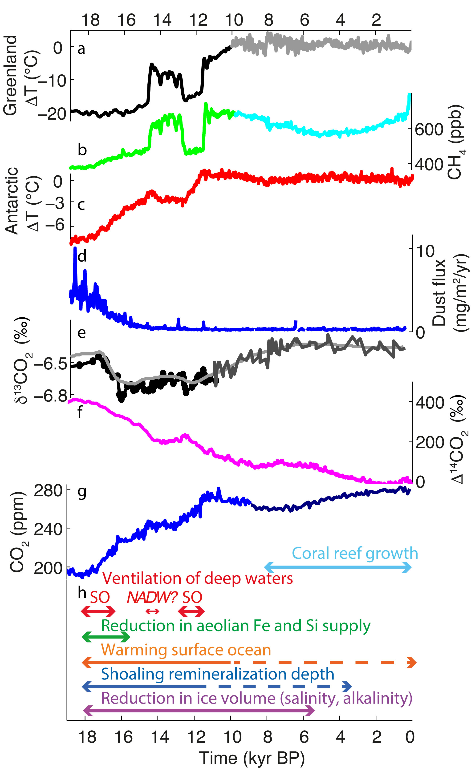
Figure 1: Timeseries of (A) Greenland surface air temperature anomalies, (B) atmospheric CH4 concentrations, (C) Antarctic surface-air-temperature anomalies, (D) dust flux, (E) δ13CO2, (F) ∆14CO2, (G) CO2, (H) estimated time span of processes discussed in text; SO stands for ventilation of Southern Ocean, NADW for deepening of North Atlantic Deep Water. References are given in the online version of this article (doi.org/10.22498/pages.27.2.60). |
A rather simple math question
While part of the glacial terrestrial carbon on exposed continental shelves was lost due to flooding (182-266 petagram carbon (PgC); Montenegro et al. 2006), CO2 fertilization, generally warmer and wetter conditions, and the newly available land under retrieving ice sheets were conducive to an overall increase in terrestrial carbon during the deglaciation. Recent estimates of net reservoir changes based on global mean ocean δ13C suggest a 300 to 460 PgC increase across the last deglaciation (Menviel et al. 2017), or even higher (~850 PgC; Jeltsch-Thömmes et al. 2019).
To account for the increase in atmospheric CO2, the ocean must therefore have released a total of ~500 to 1050 PgC across the deglaciation, of which ~190 PgC led to the observed increase in atmospheric CO2 and 300 to 850 PgC were fixed on land. How did the ocean pull this off?
There is plenty of carbon in the ocean. The modern ocean is estimated to contain ~38,000 PgC (Ciais et al. 2013), making the glacial-interglacial change a mere 1-3% of reservoir change. This rather small change – from an oceanic point of view – had large effects on the climate system. It was likely caused by a combination of the physical, biological, and chemical processes detailed below (Fig. 2). However, no state-of-the-art climate model has been able to simulate the full amplitude of change so far and the sequence of events is still poorly constrained. We have not (yet) been able to solve our rather simple math problem.
 |
|
Figure 2: Best estimates of processes contributing to atmospheric CO2 changes during the deglaciation. Dark arrows indicate high level of scientific understanding, light arrows indicate medium to low level of scientific understanding. Estimates are discussed in the text or in references in the online version of this article (doi.org/10.22498/pages.27.2.60). |
Physical and chemical processes
Given that CO2 is more soluble in cold than warm water, some of the marine carbon release can be explained by ocean warming during the deglaciation (~+25 ppm; Kohfeld and Ridgwell 2009; Ciais et al. 2013). Melting ice sheets add freshwater to the ocean, decreasing salinity, which would have partly counteracted the temperature solubility effect (~-6 ppm; Kohfeld and Ridgwell 2009). This process also decreases ocean alkalinity and DIC concentrations. Such a decrease in alkalinity decreases the solubility of CO2; however, decreasing alkalinity and DIC at a 1:1 ratio leads to an increase in solubility (~-7 ppm; Kohfeld and Ridgwell 2009). Changes in pressure due to rising sea levels and a decrease in deep-ocean alkalinity would have led to changes in the accumulation/dissolution rates of calcium carbonate in marine sediments, which is a negative feedback, and has a tendency to restore carbonate ion concentrations, and therefore alkalinity. Furthermore, the effect of weathering on land would have led to a small drawdown of atmospheric CO2, mitigated by changes in the carbonate compensation depth.
Biological processes
Some of the surface's dissolved inorganic carbon (DIC) is removed by photosynthesis and transformed into organic carbon. A small percentage of this organic carbon is exported into deeper layers and remineralized into DIC. The strength of this "soft tissue pump" depends on the net primary productivity, which is a function of temperature, nutrient and light availability, competition between species, and the Redfield ratios of the species in question. Nutrient availability depends on ocean circulation and on external fluxes of micronutrients, such as aeolian iron or silica fertilization from dust. For example, the net effect of decreasing dust deposition during the deglaciation has been estimated to have contributed ~+19 ppm to the CO2 rise (Lambert et al. 2015). The strength of the "soft tissue pump" also depends on the remineralization depth of organic carbon. This is a function of the particles' sinking speed and the remineralization rates in the deep ocean. A shoaling of the remineralization depth could have led to a +20 to +30 ppm increase in CO2 (Kwon et al. 2009; Matsumoto 2007; Menviel et al. 2012), but large uncertainties remain.
Calcifying organisms form CaCO3 shells or skeletons in addition to their soft tissue. The calcification process removes alkalinity from surface waters and increases alkalinity at depth upon dissolution. A decrease in surface alkalinity reduces the ability of surface waters to dissolve carbon; this pump has therefore been termed the "carbonate counter pump". Any changes in the competition between calcifying and non-calcifying organisms during the deglaciation, for example due to changes in silicic acid or iron availability, would have changed the strength of the combined biological pump (Matsumoto et al. 2002). In addition, a protective calcite shell changes the sinking speed of particles and thus the remineralization depth. The flooding of continental shelves increased the habitat of calcifying coral reefs, decreasing alkalinity and contributing to the Holocene atmospheric CO2 increase (~+12 ppm; Kohfeld and Ridgwell 2009).
Tying it all together: Ocean circulation
Ocean circulation connects all of the processes mentioned above in a complex way. It transports nutrients to the surface for biological carbon fixation. It also determines the residence time of deep water masses and therefore the total accumulation of remineralized carbon in the deep ocean. While much emphasis has been put on understanding North Atlantic circulation changes (e.g. Ritz et al. 2013; Huiskamp and Meissner 2012), it has recently become clear that the Southern Ocean, where most of surface/deep-water exchange takes place, is likely a more important player. Changes in Southern Ocean circulation can be prompted by changes in winds, sea-ice cover, and meridional density gradients, all of which took place during the deglaciation (Menviel et al. 2018). Finally, the Pacific Ocean is not only the largest ocean basin, it is also characterized by very sluggish circulation and therefore a much higher DIC content than any other ocean basin. Any small increase in ventilation in this basin has the potential to dramatically increase atmospheric CO2 concentrations (Menviel et al. 2014; Rae et al. 2014).
What are the models missing?
Although there has been considerable progress in carbon cycle modeling over the past 20 years, we still do not understand, nor are able to accurately simulate, all of the observed changes during the last deglaciation.
The main culprit is likely an insufficient representation and understanding of changes in ocean circulation. As discussed above, deep water masses are supersaturated in old carbon, holding 100 times more carbon than needed to explain the glacial-interglacial changes. Small circulation changes can result in considerable follow-on effects on ocean-air carbon fluxes.
So far, only models of intermediate complexity have been able to study the sequence of events leading to changes in glacial-interglacial atmospheric CO2. The spatial grids of these models are coarse and do not resolve small-scale processes in the ocean that are potentially important. While they capture the main changes in water masses well enough, they are overall too diffusive. Models that are better skilled in representing physical circulation changes, such as eddy-resolving models, cannot be integrated long enough to even get today's deep ocean circulation into equilibrium, let alone today's marine carbon cycle. Simulating a full transient deglaciation with such models is still far beyond the horizon with today's available computer power. However, these models can be used to test single processes under idealized and fixed boundary conditions.
Another culprit is most certainly the representation of ecosystems in our climate models. These model components are still in their infancy. They are highly simplified, representing the whole complexity of marine life with a few functional types for plankton based on simple equations for population dynamics. Carbon uptake, the sinking speed of particles, and remineralization rates are underconstrained and therefore overtuned (Duteil et al. 2012). It is questionable whether these models' ecosystem sensitivities can be trusted under boundary conditions that are significantly different from present-day conditions.
Finally, none of our state-of-the-art climate models include the whole complexity of sediment feedbacks, which played a non-negligible role during the deglaciation.
How do we solve this?
The proxy community is providing an increasingly coherent picture of deglacial changes. For example, recent high-resolution atmospheric CO2 and isotope records from Antarctic ice cores have highlighted the millennial variability and timing of the deglacial atmospheric CO2 increase and potential source reservoirs (Fig. 1). At the same time, the modeling community is simulating the deglaciation, or parts of it, with models of increasing complexity and higher resolution. The ultimate goal in the not-so-distant future is a transient deglacial modeling framework based on high-resolution models including high-complexity ecosystem models and sediment feedbacks to refine the sequence of the events and processes involved in the deglacial atmospheric CO2 increase.
affiliations
1Climate Change Research Centre, University of New South Wales, Sydney, Australia
2ARC Centre of Excellence for Climate Extremes, University of New South Wales, Sydney, Australia
contact
Katrin Meissner: k.meissner unsw.edu.au
references
Duteil O et al. (2012) Biogeosciences 9: 1797-1807
Huiskamp WN, Meissner KJ (2012) Paleoceanography 27: PA4296
Jeltsch-Thömmes A et al. (2019) Clim Past 15: 849-879
Köhler P et al. (2017) Earth Syst Sci Data, 9: 363-387
Kwon EY et al. (2009) Nat Geosci 2: 630-635
Lambeck K et al. (2014) P Natl Acad Sci USA 111: 15296-15303
Lambert F et al. (2015) Geophys Res Lett 42: 6014-6023
Marcott SA et al. (2014) Nature 514: 616-619
Matsumoto K et al. (2002) Global Biogeochem Cy 16: 1031
Matsumoto K (2007) Geophys Res Lett 34: L20605
Menviel L et al. (2012) Quat Sci Rev 56: 46-68
Menviel L et al. (2014) Paleoceanography 29: 58-70
Menviel L et al. (2017) Paleoceanography 32: 2-17
Menviel L et al. (2018) Nat Comm 9: 2503
Montenegro A et al. (2006) Geophys Res Lett 20: L08703
Rae JWB et al. (2014) Paleoceanography 29: 645-667
Ritz SP et al. (2013) Nat Geosci 6: 208-212
figure 2
Meissner KJ (2007) Geophys Res Lett 34: L21705