Putting the time in time machine: Methods to date ice cores
Kaden C. Martin![]() 1, S. Barnett2, T.J. Fudge3 and M.E. Helmick
1, S. Barnett2, T.J. Fudge3 and M.E. Helmick![]() 4,5
4,5
The depth–age relationship of an ice core is critical to its interpretation; it constrains rates of change and allows for comparisons among records. Chronology advancements will be critical to the investigation of new ice cores over the coming decades.
Ice cores provide remarkable insight into past environmental change. As snow falls on glaciers and ice sheets, it traps things like past air, dust, volcanic ash, and soot from fires (Wendt et al. p. 102; Banerjee et al. p. 104; Brugger et al. p. 106). These environmental indicators are preserved in the ice sheet as fresh snow falls on the surface. By drilling down into an ice sheet or glacier (Davidge et al. p. 98), researchers can travel back in time to determine what the climate was like when the snow fell. However, placing these environmental indicators into a global climate context critically relies on our ability to date these ancient layers.
To better understand the time held within ice, ice-core scientists create chronologies. A chronology defines the relationship between time and depth in ice. Like counting tree rings, physically distinct layers and chemical impurities in ice correlate to seasons. These layers are well preserved as an ice sheet grows, aiding in the production of highly-resolved and well-constrained chronologies. To create the time–depth relationship, ice-core scientists rely on a range of techniques including measurements of distinct layers, comparisons with other well-dated records, physics models of snow compression and ice flow, and radiometric dating.
Chronology fundamentals
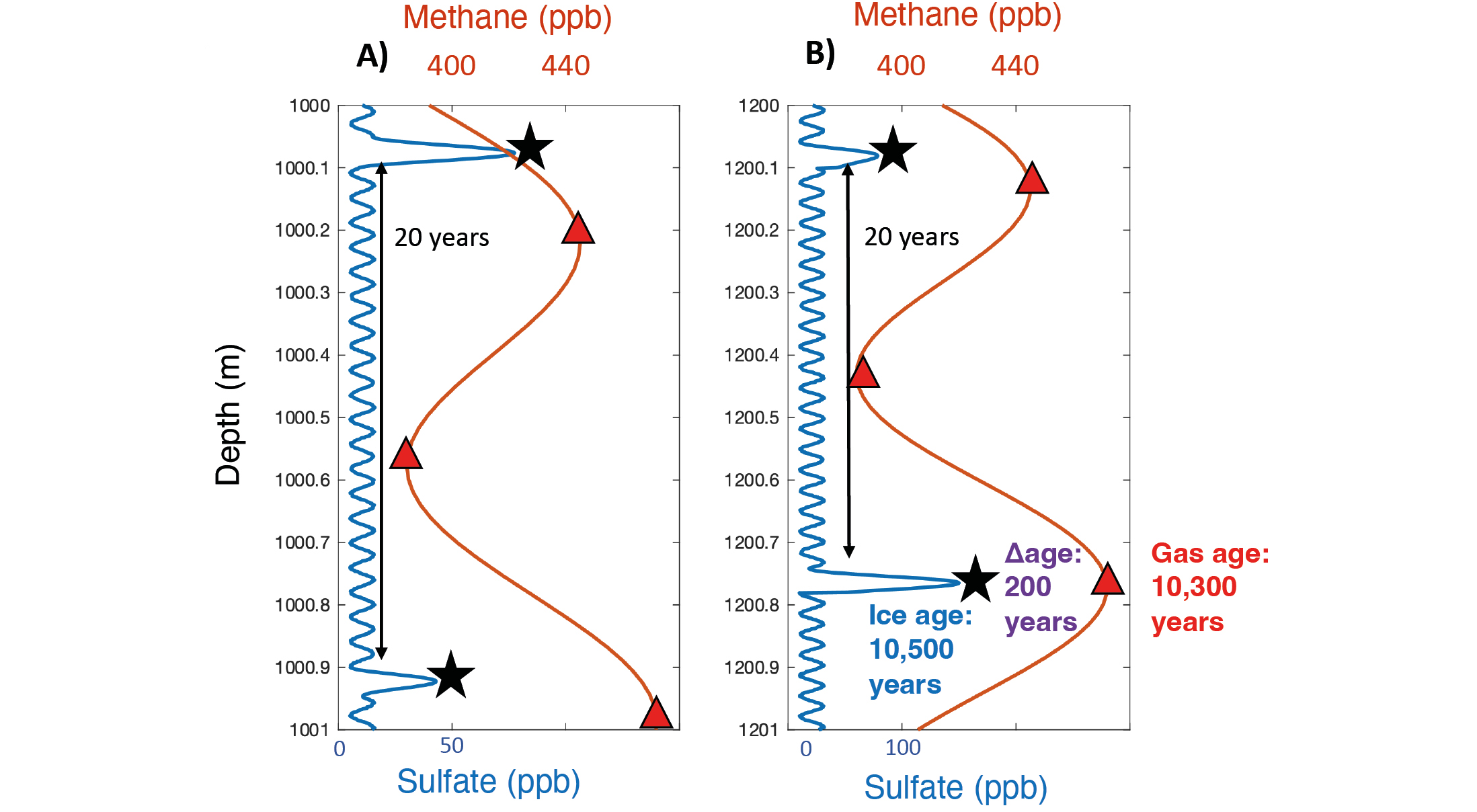
An intuitive method to develop an ice chronology is via annual-layer counting, where seasonally varying compounds or properties of ice can be used to identify yearly cycles (Fig. 1). Water isotopes, dust, and conductivity are commonly used to achieve this (Andersen et al. 2006; Sigl et al. 2016). Physical properties of ice also aid in this stratigraphy, such as visually distinct winter and summer layers due to extreme polar seasons. Annual layers become thinner with depth due to large-scale ice flow, reducing temporal resolution. Deep within an ice sheet, just a few meters can contain thousands of years of snowfall. Here, other techniques must be used as annual layers become indiscernible and dating becomes challenging.
 |
|
Figure 1: (A, B) Two idealized ice-core records, showing annual layers and volcanic events of sulfate in ice (blue) and methane concentrations in gas (orange). Annual cycles of sulfate can be counted to produce an ice chronology, while methane features can be dated using a firn model reconstruction of Δage or by examining abrupt events. The ages of cores A and B are synchronized by volcanic signals (black stars) and methane features (red triangles). Δage can be calculated between distinct features, and is 200 years in (B). |
Chronological information can be shared between cores by matching evidence of abrupt geological events. During volcanic eruptions, ash and sulfate can be deposited onto the ice sheets. These distinct layers are then preserved in the ice. If the same layer is found in different ice cores, the age of that layer can be transferred between them (Fig. 1a, b). This technique has been used to synchronize the ice chronologies of cores from Greenland and Antarctica at these discrete tie-points (Seierstad et al. 2014; Svensson et al. 2020).
A unique challenge of ice-core chronologies is that the ice crystals and the air bubbles trapped between them have different ages. Near the surface, air can move through spaces between grains of snow. This movement of air stops at the snow–ice transition, at ~40–120 m depth (McCrimmon et al. p. 112). At this point, pathways for air have closed and bubbles are sealed in ice, becoming isolated from the atmosphere. Therefore, the ice is older than the gases trapped within. This means that two chronologies are needed—one to study the ice, and one to study the gases.
The age difference between ice and gas at the same depth is Δage ("delta age"). This age difference is not the same everywhere, nor is it constant for a given core. This is because Δage responds to changes in how fast snow turns into ice, which is set by local temperature and snowfall rate (Schwander et al. 1997).
As trapped air is younger than the ice surrounding it, dating gases requires different techniques. Because Δage is the ice–gas age difference, Δage and ice chronologies can be utilized to produce gas chronologies. Δage is accurately estimated during abrupt climate change events due to distinct features that occur in environmental indicators of both gas and ice (Buizert et al. 2015). During time periods without abrupt events, Δage is estimated by modeling the physics of snow compression, emulating how snow turns into ice given the climatic conditions at the time. Estimated and modeled Δages alongside annual-layer-counted ice chronologies are then used to calculate the gas chronology. Gas chronologies are also often dated using methane (CH4). Due to rapid atmospheric mixing of CH4, its atmospheric concentration is similar everywhere in Earth's lower atmosphere at any given time. This means that changes in one core can be matched to the same change in another core (Blunier and Brook 2001). This allows for the most accurate gas chronology to be transferred to any ice core (Fig. 1b, c).
As the array of well-dated ice cores and chronological information increases, data inversion techniques can be used to establish tie-points between different cores and bring their chronologies into agreement (Lemieux-Dudon et al. 2010). Such projects have successfully supported Antarctic chronologies (Parrenin et al. 2015). The key to data inversion is to utilize all available age constraints, like volcanic events, CH4 matches, and annual-layer counts, in a mathematical framework. The framework then calculates a chronology that is within the bounds of the uncertainties and physical properties of the available data. This is a powerful technique, as it can overcome shortcomings of individual methods and reduce the time needed to construct new chronologies for recently recovered cores.
Dating the oldest ice
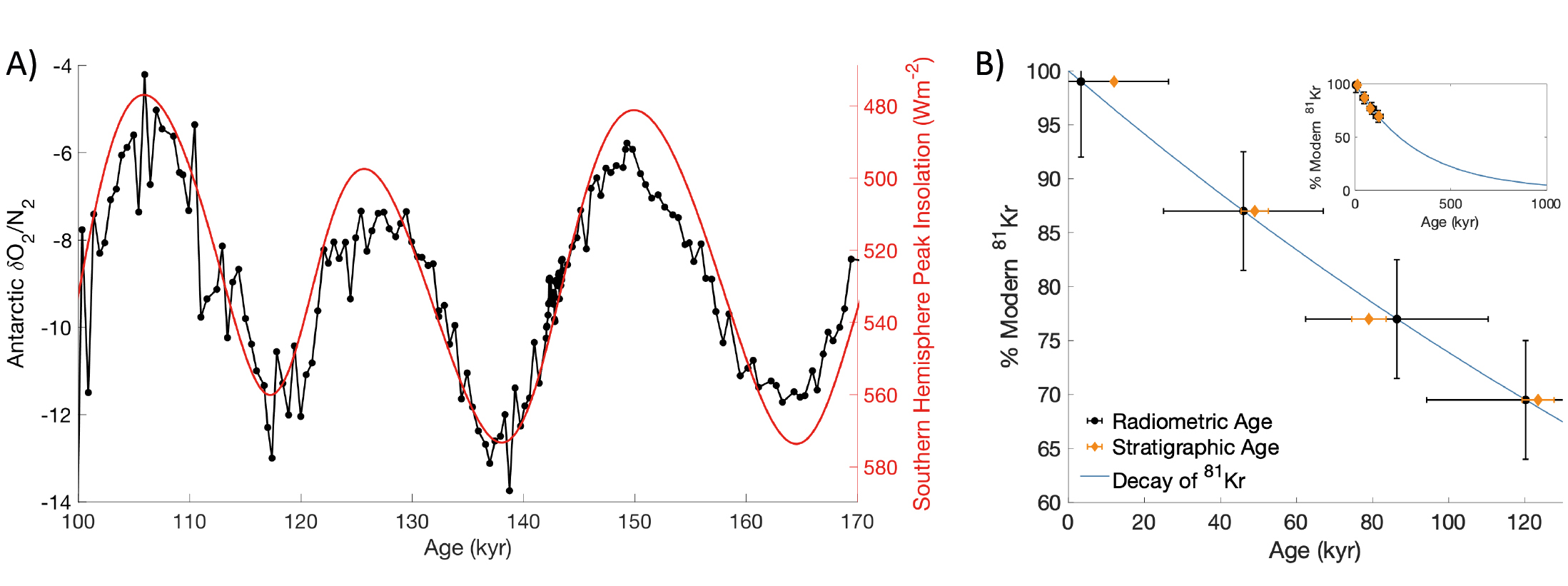
The oldest continuous ice-core records, found primarily in the East Antarctic Ice Sheet, have been dated by orbital tuning. This technique is necessary where annual layers become indistinguishable. Orbital tuning utilizes the known relationship between a proxy, like δO2/N2, and the cyclical variation of sunlight due to Earth's orbital cycles (Fig. 2; Oyabu et al. 2021). This method has been widely applied to marine sediment cores, where the variations in oxygen isotopes can be linked to changes in solar insolation and ice volume (Imbrie and Imbrie 1980).
 |
|
Figure 2: (A) The oxygen-to-nitrogen ratio (δO2/N2, black; Oyabu et al. 2021), measured from the Dome Fuji Ice Core in East Antarctica, and Southern Hemisphere peak summer sunlight, or insolation (red, note reverse axis; Laskar et al. 2004). The snow–ice transformation rate influences the δO2/N2, and this process correlates well with the location's amount of summer sunlight. By comparing δO2/N2 to past sunlight, age can be approximated. (B) Decay rate of 81Kr (blue), and the comparison between conventional dating techniques (orange) and measurements of 81Kr (black; Buizert et al. 2014). Inset: Same as in (B), but scaled to cover this technique's effective range. |
Another technique for dating old ice utilizes radiometric dating, where the known decay rate of radioactive isotopes in preserved bubbles can be used to determine when they were isolated from the atmosphere. Two useful radioisotopes are Argon-40 (40Ar) and Krypton-81 (81Kr). 81Kr is produced in the atmosphere by cosmic-ray interactions with the stable isotopes of Kr. As the atmospheric concentration of 81Kr has been relatively constant over the last 1.5 million years, a measurement of an old sample will be less than the modern concentration due to radiometric decay. The difference in concentration between an old and modern sample is set by the decay rate of 81Kr, and can be used to determine when the gas in the sample was trapped in the ice. The half-life of 81Kr is 229 kyr BP, providing a dating range of 0.5 to 1.5 million years—useful when dating old ice (Fig. 2). Ar isotopes in ice cores record the decay and outgassing of radioactive potassium in the mantle, which provides a unique chronologic marker (Bender et al. 2008).
Outlook
Chronologies are critical to placing ice-core records into a global context, enabling direct comparisons between natural greenhouse-gas variations and records of environmental change in other archives. Chronology development is an ever-growing field, supported by advancements in instrumentation, new chemical measurements, and mathematical models as past cores are updated and new projects are planned. Techniques for absolute dating are being developed to support deep ice-core projects targeting continuous climate records of 1.5 million years, such as the new COLDEX and BeyondEPICA projects, and discontinuous climate records from blue-ice areas, like Allan Hills, Antarctica (Kehrl et al. 2018).
affiliations
1College of Earth, Ocean, and Atmospheric Sciences, Oregon State University, Corvallis, USA
2School of Earth and Sustainability, Northern Arizona University, Flagstaff, USA
3Department of Earth and Space Science, University of Washington, Seattle, USA
4School of Earth and Climate Science, University of Maine, Orono, USA
5Climate Change Institute, University of Maine, Orono, USA
contact
Kaden C. Martin: martkade oregonstate.edu
references
Andersen KK et al. (2006) Quat Sci Rev 25: 3246-3257
Bender ML et al. (2008) Proc Natl Acad Sci USA 105: 8232-8237
Blunier T, Brook EJ (2001) Science 291: 109-112
Buizert C et al. (2014) Proc Natl Acad Sci USA 111: 6876-6881
Buizert C et al. (2015) Clim Past 11: 153-173
Imbrie J, Imbrie JZ (1980) Science 207: 943-953
Kehrl L et al. (2018) Geophys Res Lett 45: 4096-4104
Laskar J et al. (2004) Astron Astrophys 428: 261-285
Lemieux-Dudon B et al. (2010) Quat Sci Rev 29: 8-20
Oyabu I et al. (2021) Cryosphere 15: 5529-5555
Parrenin F et al. (2015) Geosci Model Dev 8: 1473-1492
Schwander J et al. (1997) J Geophys Res Atmos 102: 19,483-19,493
Seierstad IK et al. (2014) Quat Sci Rev 106: 29-46