Tipping ice ages

Michel Crucifix

>Access contents of this issue

>Download this article as pdf

Past Global Changes Magazine

24(1)

6-7

2016

https://doi.org/10.22498/pages.24.1.6

Michel Crucifix

Simple models formulated in the 1960s started a research tradition focused on stability and transitions in the climate system. Later, climate scientists realized the importance of stochasticity. What do these concepts imply for ice ages today?

In 1969, M.I. Budyko in Russia and W.D. Sellers in the US published two very similar studies. From reasoning about the energy balance of the Earth's system, they found that comparatively small variations of atmosphere transparency (Budyko) or in solar constant (Sellers) would be enough to drive the Earth into an ice age. Their key discovery was that Earth's climate could exhibit two steady states. Earlier that decade, Stommel (1961) deduced the existence of irreversible transitions between two thermohaline circulation structures in a simple model of abyssal water flow. Now we also think that vegetation-atmosphere coupling can lead to multiple states (Brovkin 1998).

The existence of multiple steady states leads naturally to the concept of “tipping”. Within a state, a system is largely self-stabilizing, but too large a perturbation may shift it into another self-stabilizing state, with little probability of escaping back to the original state. The ideas behind the models of Budyko, Sellers and Stommel provided a basis to interpret a range of paleoclimate events, including glacial inception, Heinrich events, and the end of African Humid Period.

What about the deglaciation? In a quite mathematical but pioneering article, Saltzman and Verbitzky (1993) pointed out that two possible destabilization mechanisms could be at play: the mechanical collapse of Northern Hemisphere ice sheets and the abrupt release of CO2 accumulated in the deep ocean to the atmosphere. These two processes are still considered relevant today (Abe-Ouchi et al. 2013; Paillard and Parrenin 2004)

Tipping to ping pong

Is the deglaciation, however, really the consequence of passing a “tipping point”? Or, to paraphrase Crowley (2002), are we looking obsessively for "tipping, tipping everywhere"?

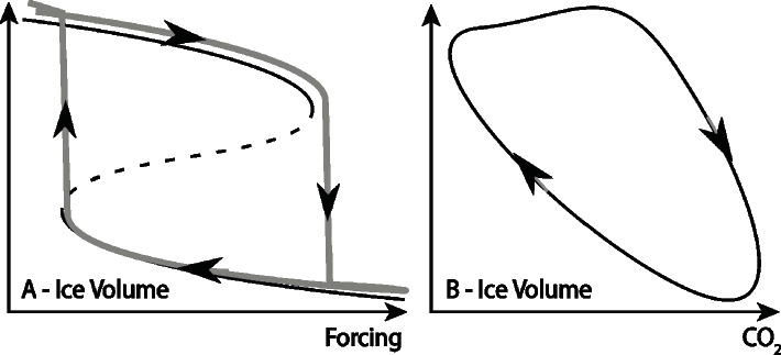
Figure 1: Two examples of conceptual models for paleoclimate dynamics. (A) The Budyko-Sellers model envisions two stable states for a range of forcing. Large forcing deviations from the resting state may precipitate a transition; (B) In a limit cycle, glacial interglacial stages succeed each other as a result of internal dynamics, without the need for forcing. In this case, insolation forcing is but a pacemaker that controls the timing of transitions.

Models such as Stommel’s feature a specific mathematical property, known in the specialized literature as a "fold bifurcation". It is a common feature of non-linear systems that fits well with the idea that a slow change in environmental conditions can induce a rapid and irreversible transition towards a new state once a "threshold" is crossed (Fig. 1A). However, this is only one of a very rich set of possibilities. For example, in the Paillard-Parrenin model (2004), a glacial maximum is inherently unstable, and CO2 outgassing ejects the system toward an interglacial. A background glaciation process then brings the system back to a glacial state, from where it is ejected again. In this model, the glacial-interglacial process no longer requires an externally forced tipping: it is the manifestation of a self-sustained oscillation, also known as a limit cycle. Instead of tipping, this (Fig. 1B) is ping pong!

Accounting for Randomness

Fold bifurcations and limit cycles are examples of concepts defined by a branch of mathematics called "dynamical systems theory". Since the 1960s, this discipline has provided climate scientists with an inexhaustible framework for depicting, characterizing and hypothesizing about possible system transitions and cycles. Ghil (1976) wrote one of the pioneering papers on the subject. More recently, Crucifix (2013), and Aswhin and Ditlevsen (2015) have analyzed models akin to those shown in Figure 1 in the context of ice ages.

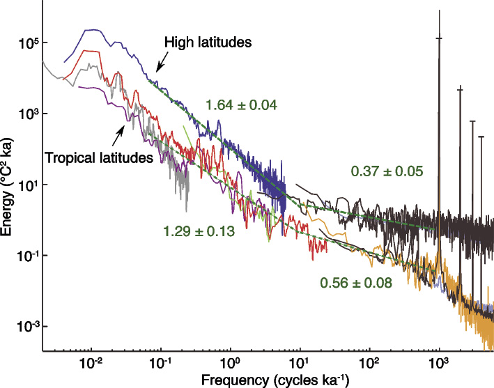
Figure 2: Estimate of the energy spectrum from annual to astronomical scales, adapted from (Huybers and Curry 2006). Numbers in green are spectral slopes on the logarithmic plot. All time scales may potentially interact: there is no gap between astronomical and centennial time scales.

Such models represent a very small class of possibilities. In particular, they are "deterministic": the trajectory is entirely determined by original conditions and forcing. Since the seventies, however, climate scientists have realized that this framework needs to be extended. The problem is that spectral analysis shows that the climate system varies on all timescales (Fig. 2), yet deterministic models always neglect a part of this spectrum. So we need, somehow, to account for the unresolved fluctuations to realistically represent dynamical effects.

This is where stochastic theory can help. A stochastic quantity is a mathematical concept used to represent a variable which is not known precisely, but which can be described in terms of probability distributions. The idea is to account for atmospheric variability with a stochastic process taking different random values with time (Hasselman 1976; Saltzman 1981).

This leads to an interesting mathematical problem: what happens to tipping points when stochastic terms are included? With small amounts of stochasticity, the system may exhibit "early warning signals" before a transition: a valuable property, indeed, if we want to predict the occurrence of a large transition. In some cases, however, the presence of stochastic components modifies the structure of the deterministic model so drastically that the tipping point completely vanishes. In this case, systems like the one depicted in Figure 1 lose their relevance. We do not know whether this scenario applies to ice ages, but in some models even small amounts of stochasticity can substantially modify the timing of ice ages (Ditlevsen 2009; Crucifix 2012).

Some will say that Nature isn't "chaotic", "deterministic", or "stochastic". These properties only apply to models. What mathematics has to offer us is the ability to characterize the model which, among alternatives, best explains the data at hand about the real world. If this best model presents tipping points, then we can take decisions accordingly.

Identifying a “best” model among alternatives is a problem that can be framed statistically. In general, statistics work best with models that do not include too many parameters. A simple model is also easier to analyze and characterize. This is why there is still a research tradition focused on conceptual models similar to those of Figure 1.

However, our knowledge of environmental systems relies also on complex numerical models, which allow us to infer emergent constraints on the basis of physical laws of ice, atmospheric and oceanic motion, and such models tend to include hundreds of parameters. A key challenge for climate scientists is thus to articulate models of different levels of complexity within a consistent framework, from the conceptual models to the complex numerical codes.

A challenge for the decade

Stochastic theory may again provide a way forward. Stochastic parameterizations of interannual and interdecadal variability could be developed on the basis of experiments with general circulation models. Such parameterizations could then be included in models of intermediate complexity (EMICs) to estimate the effects of interdecadal variability on the slower modes of motion. This would provide a means to model the cascade of variability effects, from interannual to ice-age time scales: a revolution with respect to modern practices. Whether such stochastic EMICs will still present tipping points similar to those depicted on Figure 1 is an important question waiting to be answered.

affiliation

Earth and Life Institute, Université catholique de Louvain, Louvain-la-Neuve, Belgium

contact

Michel Crucifix: michel.crucifix@uclouvain.be

references

Abe-Ouchi A et al. (2013) Nature 500: 190-193

Ashwin P, Ditlevsen P (2015) Clim Dyn 45: 2683-2695

Budyko MI (1969) Tellus 21: 611-619

Brovkin V et al. (1998) J Geophys Res 103: 31613-31624

Crowley TJ (2002) Science 295: 1473-1474

Crucifix M (2012) Phil Trans R Soc A 370: 1140-1165

Crucifix M (2013) Clim Past 9: 2253-2267