Tipping points in the past: the role of stochastic noise

Zoë A. Thomas and Richard T. Jones

>Access contents of this issue

>Download this article as pdf

Past Global Changes Magazine

24(1)

4-5

2016

https://doi.org/10.22498/pages.24.1.4

Zoë A. Thomas1 and Richard T. Jones2

The analysis of paleo-environmental archives provides a mechanism for identifying systems vulnerable to abrupt change or “tipping points”. Perturbations to natural systems, so-called “stochastic noise”, can play a significant role in understanding past and future variability.

Abrupt changes or “tipping points” in environmental systems are often characterized by a nonlinear response to gradual forcing, and may have severe and wide-ranging impacts, including an irreversible shift to a new state (on human timescales). Arguably one of the best ways to identify and potentially predict threshold behavior in environmental systems is through the analysis of natural archives (paleo records). Generic rules can be used to identify early warning signals that may be identified on the approach to a tipping point, generated from characteristic fluctuations in a time series as a system loses stability.

Recently developed methods to detect these early warning signals exploit a phenomenon called “critical slowing down”. This phenomenon predicts that as a system nears a tipping point, the recovery time to its initial equilibrium after a perturbation should increase. This increase in recovery time can be measured as increasing autocorrelation and variance over a sliding window (Kleinen et al. 2003; Lenton et al. 2012). With the popularity of the free statistical software “R”, this analysis is becoming increasingly applied by the paleo community to understand mechanisms of change (for instance, Early-Warning-Signals Toolbox at http://cran.r-project.org/web/packages/earlywarnings/earlywarnings.pdf). Time-series precursors from natural archives thus have a great potential to enhance our understanding of past abrupt change and provide a means of forewarning potential tipping points. Critical in this regard is recognizing that different rates of forcing significantly influence the temporal resolution required to identify such forewarnings in paleo-environmental time series.

Linking theory to the past

While previous studies have demonstrated the value of natural archives for identifying tipping points (e.g. Dakos et al. 2008), considerable scope exists to expand this work. A major challenge is that paleoenvironmental data typically have high noise levels and a low sampling resolution, whereas theoretical early warning indicators assume only weak stochastic disturbances. When systems are characterized by high levels of stochastic noise, early warning signals may not always detect the approach of a bifurcation (defined as the point at which a system exits its stable equilibrium), since high levels of noise can mask the signal of critical slowing down.

Although the efficacy of the leading indicators (autocorrelation and variance) has been interrogated using a long time series with low noise levels (Dakos et al. 2012), the predictive ability of these indicators with strong noise and a low sampling resolution has been less well studied. Ecological literature, however, has led the way in this regard. The importance of environmental variability in the modeling of ecological systems was first emphasized by Holling (1973), who noted that stochastic noise reduced the resilience of a system. Similarly, analysis of the leading early warning indicators using a multi-species model (Carpenter and Brock 2004) found that both increased noise intensity and decreased sampling rate were found to have a strong negative effect on the ability to detect early warning signals of an impending shift (Perretti and Munch 2012).

Figure 1: Typical behavior of systems with (A) low and (B) high noise levels, and (C) an example of flickering.

Simple bifurcation models can be used to illustrate the role of stochastic noise. It is important to note that the bifurcation point (where intrinsic stability properties of a system changes) and the point at which the system actually tips are not always the same; high noise levels often tip the system before the bifurcation point is reached (Kleinen et al. 2003). Figure 1 depicts the effect of noise on the timing of the abrupt change, showing that (1) the point of tipping varies much more with a higher noise level, and (2) the point of tipping generally occurs much earlier. Early warning signals tend to be much stronger with reduced noise intensity, when the system tends to tip closer to the bifurcation point. When the noise level is too high, the system may not have time to recover from the perturbations and thus the signals of critical slowing down may not be detected.

Critical slowing down or flickering?

When multiple stable states exist and if stochastic forcing is strong enough, the system can “flicker” back and forth between two basins of attraction as the system reaches this bistable region before the bifurcation (Scheffer et al. 2009; e.g. Fig. 1c). This can be seen in the behavior of lakes prior to a switch from oligotrophic to eutrophic conditions, observed as short-term eutrophication events and algal blooms before a more long-term switch (e.g. Wang et al. 2012). Importantly, many studies which give empirical evidence of critical slowing down do so under a small amplitude of noise, which allows the system to display critical slowing down rather than flickering (Dakos et al. 2013), but is generally unrealistic in paleoenvironmental systems. Since “flickering” seems to occur when there is a high noise level, this behavior is probably more prevalent in climate systems than first thought.

An appreciation of the number of states within the system can be beneficial to understand the underlying dynamics of a system. For some time series, this can be visually obvious or is pre-determined by a theoretical model, such as Stommel’s two box model of the thermohaline circulation (Stommel 1961). The exact number of states in a system is sometimes difficult to determine by eye, however, particularly when there are more than two states present. Potential analysis is a technique that can be used to determine the number of states in a system over time, by reconstructing the changing state-space of a system through the modality of the data distribution (Livina et al. 2010). In systems with a relatively high level of noise, if there are multiple stable states present, the system is likely to sample these states over time and this represents a kind of flickering in the system (Dakos et al. 2012).

Multiple stable states: A case study

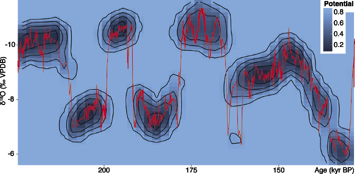
Figure 2: Visualization of the potential function derived from the speleothem δ18O data (overplotted in red; x-axis inverted), showing the presence of multiple stable states (Wang et al. 2008; Thomas et al. 2015). The potential function gives an intuitive picture of the stability of the system, where darker blue indicates a deeper, more stable potential, and the lighter blue areas an unstable region of the potential basin.

The techniques described above have been used in the analysis of speleothem sequences from China to gain an understanding of the mechanisms of abrupt changes in the Asian monsoon system (Thomas et al. 2015). Figure 2 shows the δ18O values from a speleothem from Sanbao Cave in China (Wang et al. 2008), spanning the penultimate glacial cycle. More negative δ18O values indicate higher rainfall amount (strong monsoon), while less negative δ18O values indicate lower rainfall amount (weak monsoon), over millennial timescales. Potential analysis undertaken on this data shows that the system jumps between different stable states (indicated by the darker blue areas in Fig. 2), from a strong monsoon state to a weak monsoon state and vice versa. This is particularly prominent during the older half of the record.

Conclusion

The recognition of multiple stable states in natural archives provides a powerful means of understanding Earth system dynamics. The ability to identify periods in the past where thresholds have been crossed is critical if we are to predict and avoid dangerous abrupt climate change in the future.

Acknowledgements
This work is supported by the Australian Research Council Laureate Fellowship (FL100100195). Thanks to Chris Turney and Tim Lenton for help editing this paper.

affiliations

1Climate Change Research Centre, University of New South Wales, Sydney, Australia

2Department of Geography, University of Exeter, UK

contact

Name: z.thomas@unsw.edu.au

references

Carpenter SR, Brock WA (2004) Ecol Soc 9: 8-38

Dakos V et al. (2008) PNAS 105: 14308-14312

Dakos V et al. (2012) PLoS One 7, doi:10.1371/journal.pone.0041010

Dakos V et al. (2013) Theor Ecol 6: 309-317

Holling CS (1973) Annu Rev Ecol Syst 4: 1-23

Kleinen T et al. (2003) Ocean Dyn 53: 53-63