Modeling deep ocean flow speeds and δ13C during the Last Interglacial: Towards a more direct model-data comparison
Pepijn Bakker1,2, A. Govin3, D. Thornalley4, D. Roche1,5 and H. Renssen1
Using a climate model we investigate how changes in the strength of the Atlantic Meridional Overturning Circulation (AMOC) are reflected in water flow speeds and foraminiferal δ13C, two tracers of AMOC variability commonly measured in marine sediment cores.
Investigating past changes in the Atlantic Meridional Overturning Circulation (AMOC) provides us with clues about the possible multi-decadal to centennial response of the AMOC to projected global warming. Realistic and physically consistent evidence about past changes can be obtained from combining ocean model simulations of past scenarios with real-world proxy data. The common approach for this is to qualitatively compare the model output, i.e. the simulated stream function of maximum AMOC with paleocanographic reconstructions, e.g. foraminiferal δ13C as a proxy for deep sea ventilation changes (Duplessy 1981; Shackleton 1977), or sortable silt as a proxy for bottom water flow speed (McCave et al. 1995). However, this approach is limited to being semi-quantitative at best because (i) different paleoceanographic proxies record different aspects of the AMOC and (ii) comparing these proxies to climate model outputs is not trivial since non of the proxies record the physical overturning as expressed by the stream function. We therefore simulated the water flow speed and δ13C directly within the ocean circulation model. This allows us to discuss what aspects of AMOC changes the two AMOC proxies record, and how this depends on the geographical context.
Towards more direct model-data comparisons
Full carbon cycle dynamics, including isotopes, have been developed and built into the 3-dimensional global climate model of intermediate complexity, iLOVECLIM (Bouttes et al. 2014). In our study, we focus on the Last Interglacial period (LIG; ~130-116 ka BP), which is particularly relevant to future concerns because it was characterized by significant changes in the AMOC strength (Galaasen et al. 2014, and this issue; Govin et al. 2012; Hodell et al. 2009; Oppo et al. 1997, 2006; Sânchez-Goñi et al. 2012) at global temperatures higher than today (e.g. CAPE Members 2006).
We performed a fully coupled transient simulation that covers the 132-120 ka BP time interval. We mimicked the range of reconstructed AMOC changes by gradually tuning up its strength in the model from a nearly collapsed state, to a weak state, and finally, a strong state similar to the present-day. Accordingly, the model produced changes in flow speed and δ13C.
 |
|
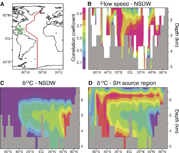
Figure 1: Correlations between AMOC driving factors and simulated flow speeds or δ13C along a vertical transect through the Atlantic. (A) Map showing the transect path (red line) and the site used in Fig. 2 (green rectangle). (B) Correlations of the flow speed with NSDW. Correlation of δ13C with (C) NSDW, and (D) SH-source region δ13C changes. The cross-section roughly follows the western boundary of the Atlantic basin. Gray shading means bottom topography; white shading means that no linear combination of the drivers yielded a correlation with the flow speed changes above 0.5. |
 |
|
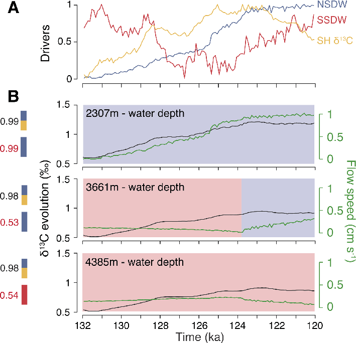
Figure 2: Comparison of the simulated evolution of AMOC indicators during the LIG and their main large-scale drivers for three water depth levels at a site (grid-cell) located in the path of the DWBC in the subtropical northwestern Atlantic (green rectangle in Fig. 1A). (A) Simulated main drivers. (B) Evolution of δ13C (black) and flow speed (green). The vertical colored bars and associated R2 correlation values indicate the relative importance of the main (normalized) drivers shown in panel A in reaching a best linear fit with the simulated records of δ13C (top bar) and flow speed (lower bar), respectively. For flow speed only NSDW and SSDW were taken into account. Red and blue shading of the panels indicate the water mass prevalent at each depth level, where southward flow was taken to be indicative of SSDW, northward flow of NSDW. |
To constrain the underlying mechanisms of flow speed and δ13C we calculated temporal correlations with several potentially important drivers. For local flow speed changes we consider two potential drivers: the transport of deep water formed in the North Atlantic (northern-sourced deep water; NSDW) and deep water formed in the Southern Ocean (southern-sourced deep water; SSDW). In addition to the transport of NSDW and SSDW, we assume that changes in local δ13C may also be driven by δ13C changes in the Northern Hemisphere or Southern Hemisphere source regions or by changes in the local export productivity of biomass from the sea surface to the interior ocean. The relative importance of the drivers is determined by maximizing the correlation for every individual grid-cell between (1) a linear combination of the drivers and (2) flow speed and δ13C respectively (Fig. 1). Only the drivers that proved important are discussed in the following and shown in Figs. 1 and 2.
Distinguishing Atlantic deep water masses
In the depth profiles in Fig. 1, the correlation coefficients between simulated δ13C and the predetermined drivers show distinguished patterns that can be associated with the main Atlantic deep-water masses. For example, δ13C values in the North Atlantic Deep Water region centered around 3 km depth appear driven by changes in NSDW (Fig. 1C), while changes in the surface water δ13C in the Southern Hemisphere region of deep water formation (SH source region, Fig. 1D) drive the δ13C evolution in the Antarctic Intermediate Waters and Antarctic Bottom Waters, centered around 1.7 km and 4.5 km respectively.
Conversely, the correlation pattern for simulated flow speed and its drivers does not reveal such clear large-scale water masses. This could indicate that flow speed changes are not reflecting large scale changes in the transport of NSDW and SSDW, however, in the following we will show that they do, and moreover, that they allow an investigation of the thickness and depth habitat of the different water masses (Thornalley et al. 2013).
Local-scale and vertical water mass changes revealed by simulated flow speed
Local flow speed changes relate to changes in the vertical structure of the water column, i.e. the migration of the boundary between the two main water masses at the site (NSDW overlying SSDW) and their thicknesses. This can be demonstrated when analyzing the LIG simulation at three depth-levels of a single model grid-cell in the core of the Deep Western Boundary Current (DWBC; Figs. 1A and 2).
At the 2307 m depth-level, NSDW predominates throughout the LIG. Accordingly, the correlation between flow speed and NSDW strength is high. Both increase almost linearly, and level off during the last few millennia of the LIG.
At the 3661 m depth-level, SSDW predominates until 124 ka BP, but as the SSDW water mass gradually migrates downwards as a result of expanding NSDW, the SSDW core region, where northward flow velocity is at its maximum, sinks away from the 3661 m depth level, resulting in a local decrease in flow speeds. At 124 ka BP, NSDW has reached the site, and as its corresponding velocity maximum gradually migrates towards the 3661 m depth-level, it causes flow speed to increase again.
At the 4385 m depth-level, SSDW predominates throughout the LIG; however, the expansion of NSDW pushes the SSDW core downwards over time. At first flow speed increases as the SSDW velocity maximum moves towards the 4385 m depth level and during the later part of the LIG flow speeds start to decrease when the SSDW velocity maximum core has passed the 4385 m depth level and moves even deeper.
Outlook
Simulating flow speeds and δ13C changes in response to a strengthening AMOC shows that the two parameters yield different but complementary information about deep ocean circulation changes: the δ13C record provides information about the large scale water mass changes, while flow speed changes relate to the vertical migration and thickness of the different deep ocean water masses.
The limitations of this study lie in the fact that (i) we use a low-resolution climate model and (ii) our methodology simplifies the complexity of the climate system by implying that the different drivers are independent from each other and that their relative contributions are constant through time.
This study provides the ground for quantitative δ13C and flow speed model-data comparison (Bakker et al. in review). Another worthwhile target for future studies of a similar design may be the deglaciation across the Younger Dryas, a period characterized by strong AMOC changes and a good density of high-resolution paleoceanographic proxy data.
affiliations
1Faculty of Earth and Life Sciences, VU University Amsterdam, The Netherlands
2College of Earth, Ocean, and Atmospheric Sciencees, Oregon State University, USA
3MARUM - Center for Marine Environmental Sciences, University of Bremen, Germany
4Department of Geography, University College London, UK
5Laboratoire des Sciences du Climat et de l’Environnement, Gif-sur-Yvette, France
contact
Pepijn Bakker: pbakker ceoas.oregonstate.edu
references
Bouttes N et al. (2014) Geosc Mod Dev Discussions 7: 3937-3984
CAPE Members (2006) Quat Sci Rev 25: 1383-1400
Duplessy JC et al. (1981) Palaeogeogr Palaeoclimatol Palaeoecol 33: 9-46
Galaasen EV et al. (2014) Science 343: 1129-1132
Govin A et al. (2012) Clim Past 8: 483-507
Hodell DA et al. (2009) Earth Planet Sci Lett 288: 10-19
McCave IN et al. (1995) Paleoceanography 10: 593-610
Oppo DW et al. (1997) Paleoceanography 12: 51-63
Oppo DW et al. (2006) Quat Sci Rev 25: 3268-3277