Late Holocene sea level

Barnett RL, Kemp AC & Gehrels WR

>Access contents of this issue

>Download this article as pdf

Past Global Changes Magazine

27(1)

8-9

2019

https://doi.org/10.22498/pages.27.1.8

Robert L. Barnett1,2, A.C. Kemp3 and W.R. Gehrels4

Late Holocene proxy-based sea-level reconstructions are key to understanding and identifying drivers of ongoing and future sea-level change. They demonstrate that the rate of 20th century global mean sea-level rise is unprecedented in, at least, the past 3000 years.

Relative sea level (RSL) varies across space (local to global) and through time (minutes to millennia). Proxy-based reconstructions provide insight into the physical processes that govern these spatio-temporal patterns of RSL change, including the distribution of land-based ice melt, glacio-isostatic adjustment (GIA) and ocean-atmosphere dynamics. They can also help to constrain projections of future RSL change under climate change scenarios. Reconstructions of late Holocene (roughly the past 3000 years) RSL changes are of limited use as direct analogues for future changes in which the magnitude of forcing will be greater and faster than climate variability during this period. Analogues for future RSL change are more likely to be found (for example) in the Pliocene (Miller et al. this issue) or the Last Interglacial (Dutton and Barlow, this issue). Nevertheless, the late Holocene is a key period for reconstructing RSL for the following reasons (e.g. Kemp et al. 2015):

• Records are available at abundant sites from polar to tropical regions, offering a uniquely (almost) global spatial coverage;
• Undisturbed geological archives (e.g. coastal sedimentary sequences and coral microatolls) provide near-continuous temporal coverage;
• Reconstructions are supported by chronologies with a high degree of temporal precision (years to decades in some cases);
• Some long-term geological processes can be considered negligible (e.g. dynamic topography) or linear (e.g. GIA) through time, helping in signal separation;
• Proxy-based reconstructions overlap, and can be combined, with instrumental RSL records from tide gauges and satellite altimetry;
• Complementary reconstructions of climate variables (e.g. temperature) allow direct comparison among proxies to gain insight into drivers, synchronicity and feedbacks in coupled systems, especially during periods of known late Holocene climate variability (e.g. Medieval Climate Anomaly, Little Ice Age and 20th century warming)

Sources of late Holocene relative sea-level reconstructions

Late Holocene RSL variability has magnitudes of tens of centimetres and timescales of decades to centuries, (although in tectonically active regions, near-instantaneous and larger-scale RSL jumps can occur from earthquake deformation). Changes on these scales are best reconstructed from intertidal wetlands (salt-marsh and mangrove sediments), coral microatolls, and archaeological remains. Reconstructing RSL relies on establishing a relationship between sea-level proxies and tidal elevation within modern environments, which are then applicable to the geological record as analogues (e.g. Shennan 2015).

Micro-organisms (foraminifera, diatoms, and testate amoebae) and geochemical signatures (for example δ13C and C/N ratios) in salt marshes and mangroves are found in elevation-dependent vertical niches within the upper intertidal zone (e.g. Barlow et al. 2013). Recognition of their fossil counterparts in dated sediment cores enables RSL to be reconstructed. In many cases, the history of sediment accumulation is established by an age-depth model constrained by radiocarbon dates and recognition of chronological horizons of known age in downcore profiles of elemental abundance, isotopic ratios and/or radioisotope activity. Coral microatolls live slightly below the intertidal zone and grow laterally during times of stable RSL, upward under conditions of RSL rise, and experience die-back (by prolonged exposure to air and direct sunlight) if RSL falls (Meltzner and Woodroffe 2015). Therefore, the architecture of dead coral microatolls records a history of RSL change that can be dated using U/Th, radiocarbon and/or counting of annual bands. Some coastal structures were designed and built to have a specific relation to sea level and can be dated using archaeological and historical context (Morhange and Marriner 2015). For example, submerged Roman fish ponds in the Mediterranean are evidence for RSL rise.

Global mean sea level (GMSL)

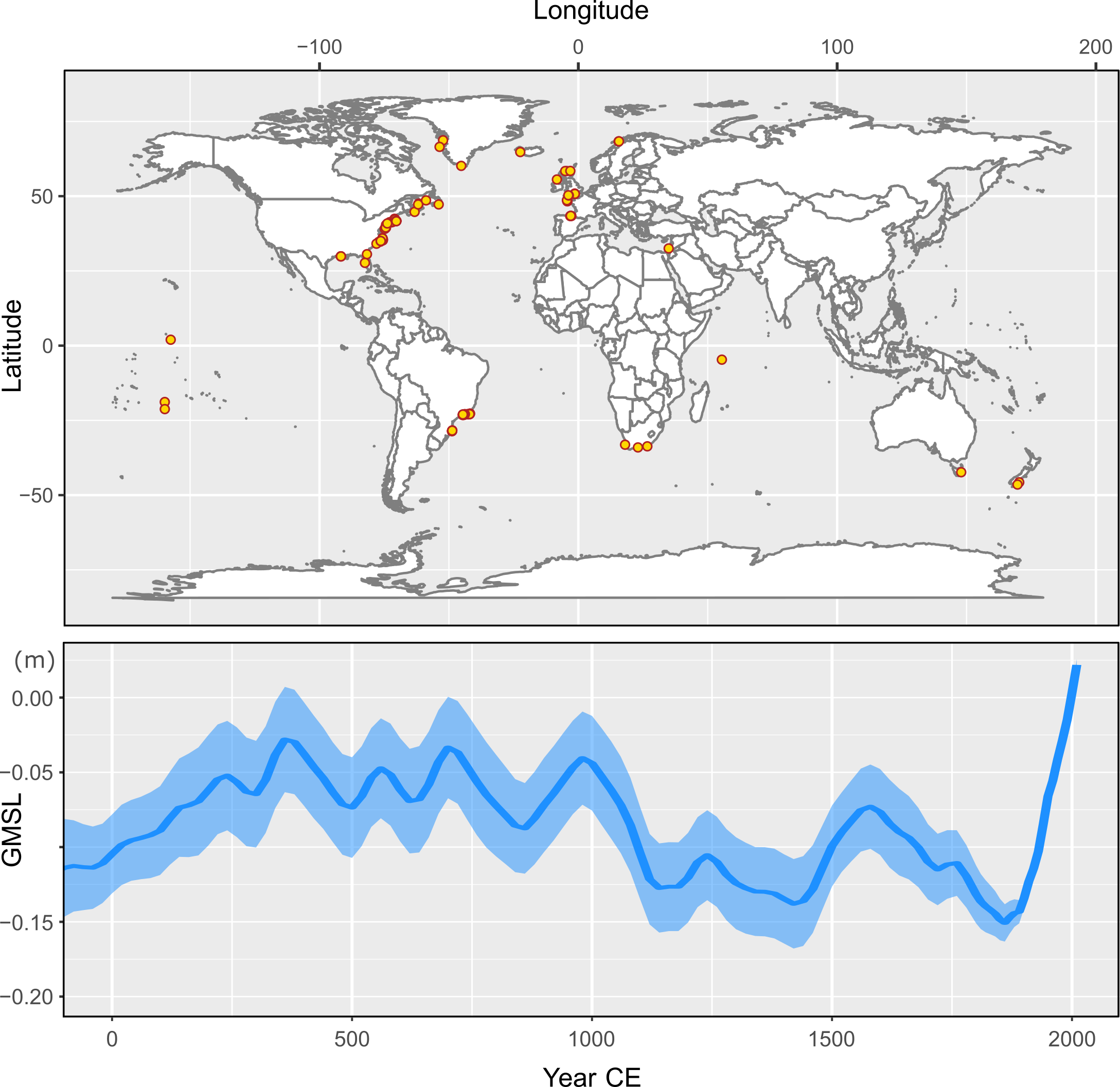
Late Holocene RSL reconstructions span the transition from geological to instrumental records and can uniquely estimate when modern rates of sea-level rise began. Tide gauges (after correction for GIA) show evidence of GMSL rise since 1880 CE, which indicates that the onset of modern rise likely predates most instrumental datasets. Proxy reconstructions from widely separated sites (Atlantic coast of North America; Australia; New Zealand; South Africa) show that RSL rise accelerated during the late 19th or early 20th century. The near-synchronous timing and wide geographic range point to a GMSL change. Kopp et al. (2016) compiled RSL reconstructions and used a spatio-temporal model to estimate late Holocene GMSL (Fig. 1). They concluded, with probability higher than 95%, that the 20th century experienced the fastest rate of rise of any century in the past ~3000 years. Their analysis also revealed a positive GMSL trend (0.1±0.1 mm yr-1) from 0 to 700 CE prior to the Medieval Climatic Anomaly and a negative GMSL trend (-0.2±0.2 mm yr-1) from 1000 to 1400 CE prior to the Little Ice Age.

Figure 1: Location of late Holocene relative sea-level reconstructions (top panel) in the database used to develop the Common Era global mean sea-level curve (bottom panel) of Kopp et al. (2016).

Calibration of semi-empirical models using the late Holocene GMSL reconstruction of Kopp et al. (2016) and global temperature reconstructions (e.g. PAGES 2k Consortium 2017) is one way in which proxy RSL reconstructions are used to constrain GMSL projections. Temperature projections from Representative Concentration Pathways are used to force the calibrated model and develop GMSL projections. When calibrated only with instrumental data, semi-empirical models often generate higher GMSL projections than process-based models (e.g. Church et al. 2013). However, calibration with late Holocene GMSL and temperature yields similar projections for semi-empirical and process-based models (Kopp et al. 2016). Using these models, Bittermann et al. (2017) explored how GMSL could change under climate scenarios that are compatible with the Paris Agreement.

Regional sea-level changes

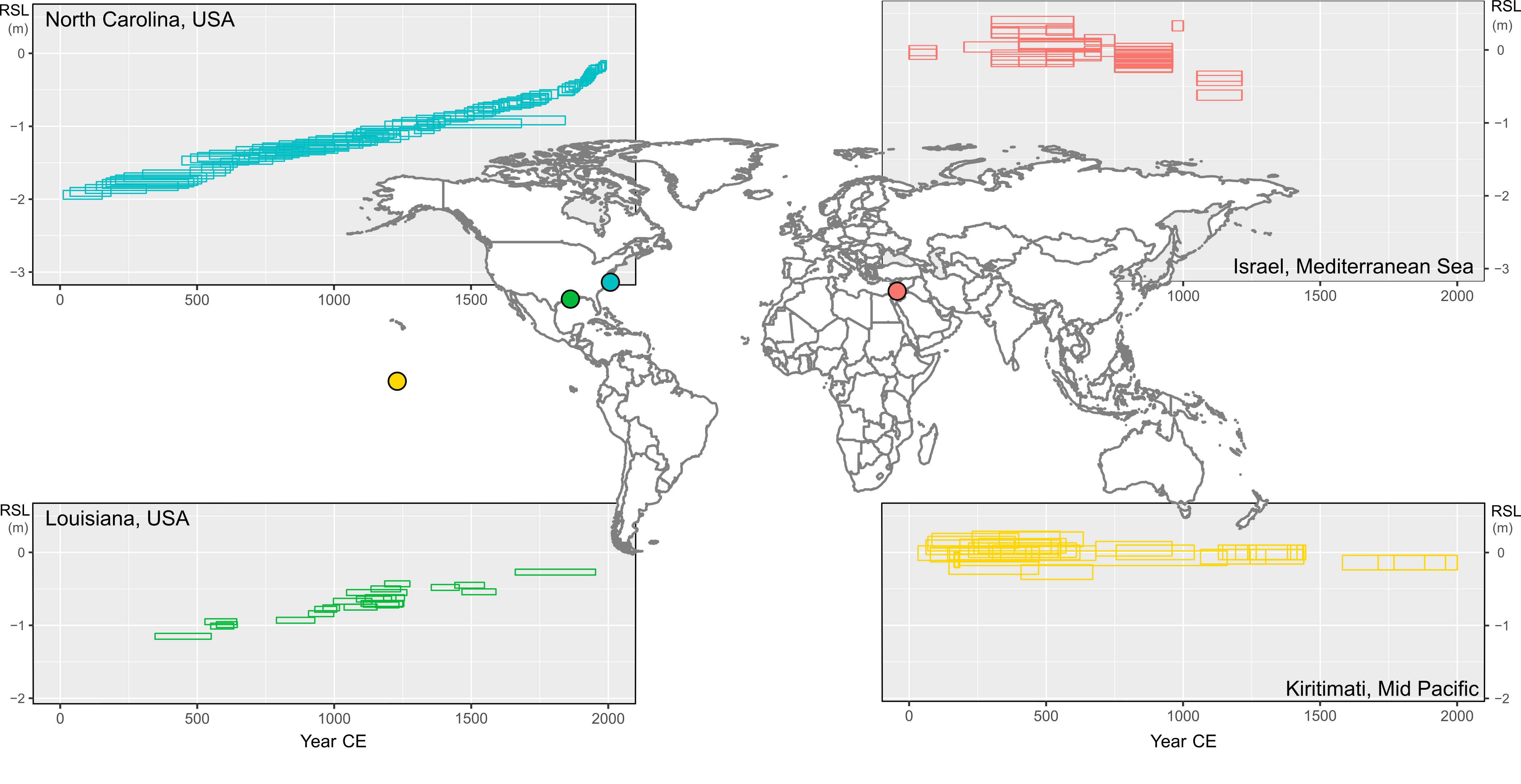
Many physical processes that drive late Holocene RSL changes produce distinctive spatial and temporal patterns. Differences and similarities among RSL records can therefore yield insight into the processes that caused late Holocene RSL change. GIA effects include crustal rebound, continental levering, ocean syphoning, and Earth rotational feedbacks from redistribution of mantle and ocean mass (Milne and Mitrovica 1998). Isostatic changes from GIA and sediment- and hydro-(un)loading of the lithosphere cause spatially variable vertical land motion that affects regional RSL signals. RSL changes resulting from Greenland, Antarctic, and glacial meltwater are also spatially variable because of reorganization of the geoid resulting in higher or lower than average RSL rise in the far or near-field respectively (Mitrovica et al. 2001). Late Holocene RSL stability reconstructed from far-field (Indian Ocean) coral microatolls on Kiritimati (Fig. 2) was used to infer minimal ice-ocean mass flux during this period (Woodroffe et al. 2012). Steric (thermal and salinity) changes cause spatially variable sea-surface height changes, although how these signals propagate from the central ocean to the coast remains poorly understood. Ocean and atmosphere circulation modes drive dynamic sea-level variations due to baroclinic gradients causing redistribution of existing ocean mass.

Figure 2: Selected late Holocene RSL reconstructions developed from salt-marsh sediment (North Carolina; Kemp et al. 2017 and Louisiana; González and Törnqvist 2009), coral microatolls (Kiribati; Woodroffe et al. 2012) and archaeological remains (Israel; Sivan et al. 2004).

Separation of RSL records into individual driver-related signals remains an active and ongoing challenge. Positive identifications are dependent on a critical spatial density of records so that local-, regional-, and global-scale signals are distinguishable. To date, this density of records only exists in the western North Atlantic Ocean (Fig. 1). Kemp et al. (2018) used a spatio-temporal model to estimate global, regional linear, regional non-linear, and local components of RSL changes with a focus on the western North Atlantic. The analysis resolves GIA effects (the regional linear component) independent from GIA models and identified regional non-linear trends that point to ocean-atmosphere dynamic forcing during the late Holocene. Addressing the spatial distribution bias of RSL records is an important and necessary step towards expanding these spatio-temporal analyses to other regions. A point of emphasis in future work should be replication of RSL reconstructions (within cores, sites and regions) to better differentiate regional RSL signals from possible reconstruction biases and local effects.

affiliations

1Coastal Zone Dynamics and Integrated Management Laboratory, University of Quebec at Rimouski, Canada
2Geography, College of Life and Environmental Sciences, University of Exeter, UK
3Department of Earth and Ocean Sciences, Tufts University, Medford, MA, USA
4Department of Environment and Geography, University of York, UK

contact

Rob Barnett: r.barnett@exeter.ac.uk

references

Barlow NLM et al. (2013) Glob Planet Cha 106: 90-110

Bittermann K et al. (2017) Env Res Lett 12: 124010

Church JA et al. (2013) IPCC AR5 WG1: 1137-1216

González JL, Törnqvist TE (2009) Quat Sci Rev 28: 1737-1749

Kemp AC et al. (2015) Curr Clim Cha Rep 1:205-215

Kemp AC et al. (2017) Quat Sci Rev 160:13-30

Kemp AC et al. (2018) Quat Sci Rev 201:89-110

Kopp RE et al. (2016) PNAS 113: 1434-1441

Meltzner AJ, Woodroffe CD (2015) In: Shennan I et al. (Eds) Handbook for Sea Level Research. Wiley, 125-145