Paleo ice-sheet modeling to constrain past sea level

de Boer B, Colleoni F, Golledge NR & DeConto RM

>Access contents of this issue

>Download this article as pdf

Past Global Changes Magazine

27(1)

20-21

2019

https://doi.org/10.22498/pages.27.1.20

Bas de Boer1, F. Colleoni2, N.R. Golledge3 and R.M. DeConto4

Numerical ice-sheet models are a key tool to estimate the contribution of ice sheets to past sea-level change. Here, we highlight a few developments and applications of ice-sheet models that allow ice-sheet contributions to past sea-level changes to be estimated.

Past warm intervals such as the mid-Piacenzian Warm Period (mPWP: 3.264-3.025 million years ago) or the Last Interglacial (LIG: 129-116 thousand years (kyr) ago) have been widely studied to constrain past sea-level changes (e.g. Sutter et al. 2016; de Boer et al. 2017). Also, those intervals are studied for process understanding of the Earth system as an analogue for future warming (e.g. DeConto and Pollard 2016). Geological evidence indicates that global mean sea level during the mPWP and LIG were likely to be up to 20 m or more (Miller et al. 2012) and 6-9 m (Dutton et al. 2015) relative to the present, respectively. This reflects the cumulative (a)synchronous contribution of the Greenland and Antarctic ice sheet (GrIS and AIS). Numerical ice-sheet models are the only means to determine their individual contribution to past sea-level changes.

Ice sheets in the climate system

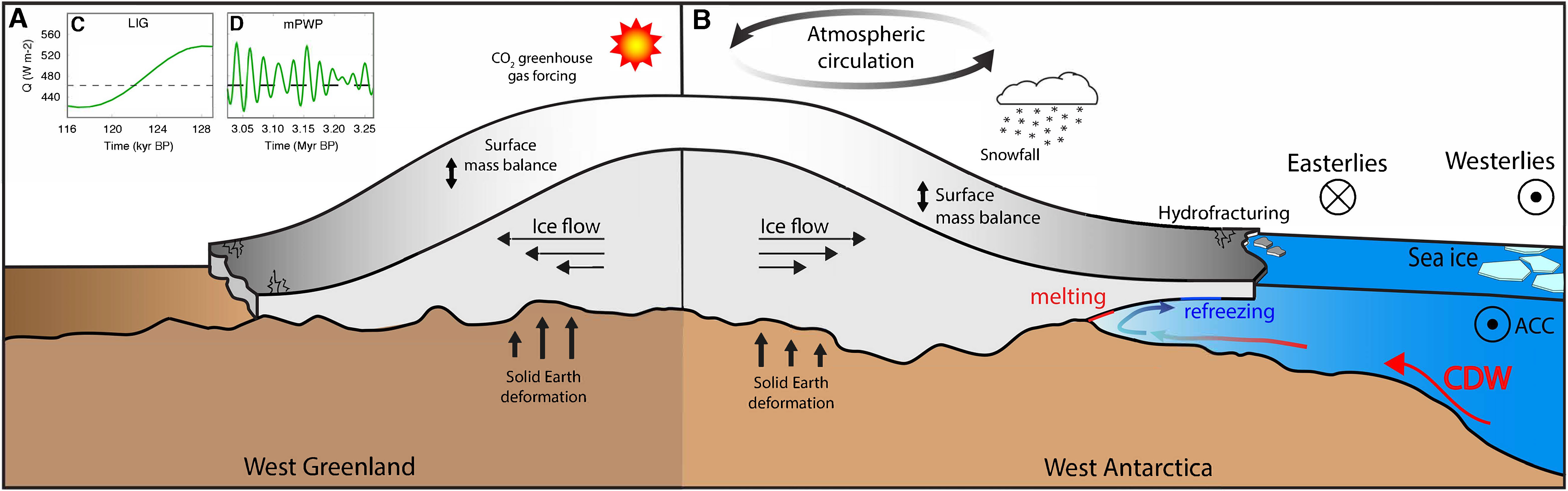
Over the past decades, critical aspects of ice-sheet models related to the interactions with the ocean, the atmosphere, basal hydrology, and the solid Earth, have been substantially improved. The mass budget of the ice sheets is largely affected by processes that act at the interface between these different systems (Fig. 1). Of the present mass budget of the GrIS, surface melting accounts for 60% of the mass loss (van den Broeke et al. 2016). During the mPWP (besides increased greenhouse gases) and the LIG, higher summer insolation (Fig. 1c,d) can increase mass loss significantly and induce ice-sheet retreat (e.g. Robinson and Goelzer 2014; de Boer et al. 2017).

Figure 1: Schematic representation of an ice sheet that (A) terminates on land. Heavy crevassing at the edges, insolation, snowfall, and temperature control the mass balance. (B) Schematic of an ice sheet that terminates at the ocean. Melting at the grounding line is induced due to intrusion of CDW in the cavities underneath the ice shelves. Hydrofracturing and sub-shelf melting dominate the mass balance of ice shelves that buttress the ice sheet. Inset shows insolation at June 65°N (Laskar et al. 2004) during (C) the LIG (129-116 kyr ago) and (D) the mPWP (3.264-3.025 Myr ago). The horizontal dashed line shows present insolation at 462.29 W m-2.

The ocean plays a key role in AIS changes (e.g. Sutter et al. 2016; Golledge et al. 2017), largely due to the fact that large sectors of the bed lie well below sea level. Punctuated intrusion of relatively warm and saline ocean water – Circumpolar Deep Water (CDW) – underneath the ice shelves (Fig. 1b) enhances ice-shelf basal melting and thinning, leading to a significant contribution to the mass loss of ice shelves. Under warm climatic conditions, climate models show that intrusion of CDW is fostered by a southward shift and strengthening of the westerly winds, which leads to a more vigorous Antarctic Circumpolar Current (ACC), and increases sub ice-shelf melting (see also Fig. 4 in Colleoni et al. 2018).

Development of paleo ice-sheet models

The basic principles that enable the use of 3D ice-sheet models for long-term paleoclimate applications involve the adoption of approximate flow equations (i.e. the shallow ice and shallow shelf approximations). This allows for relatively fast calculations (e.g. 100 kyr in a few hours), on coarse grids of 20-40 km, of continental-scale ice sheets. Complex atmospheric or oceanic interactions would require coupling (a)synchronously with a climate model, but are still computationally too expensive. Therefore, in stand-alone ice-sheet models, atmospheric and oceanic variations are crudely parameterized, and long-term transient evolution in surface air temperatures and precipitation usually follows reconstructions of ice-core or benthic oxygen isotope records (e.g. Huybrechts 2002; de Boer et al. 2017).

To determine the surface mass balance, long-term paleo ice-sheet simulations rely on simple parametrizations of snow accumulation and surface melting. Melt can be computed using the Positive Degree Day method (PDD), which uses only temperature (e.g. Huybrechts 2002), or alternatively accounting for insolation forcing on surface melt through the Insolation Temperature Melt (ITM) model (e.g. Robinson and Goelzer 2014). PDD and ITM are computationally inexpensive parameterizations and capture the glacial-interglacial behavior of continental-scaled ice sheets, but differences can be large relative to full energy balance models (e.g. Plach et al. 2018).

Similarly, for the ice-shelf-ocean interface, long-term ice-sheet simulations rely on local heat-balance parameterizations using a vertically uniform oceanic temperature, or a spatially varying field based on present-day observations (e.g. DeConto and Pollard 2016). More complex schemes are being developed, such as plume-melt models (Lazeroms et al. 2018), which account for the interaction with the local geometry and the spatially varying oceanic temperatures, or ocean box models, directly coupled to ice-sheet models, which simulate the overturning circulation in ice-shelf cavities (Reese et al. 2018). Accordingly, model developments are critical to improve calculation of GrIS and AIS contribution to past and future sea-level variations.

Modeling past sea level from the GrIS and AIS

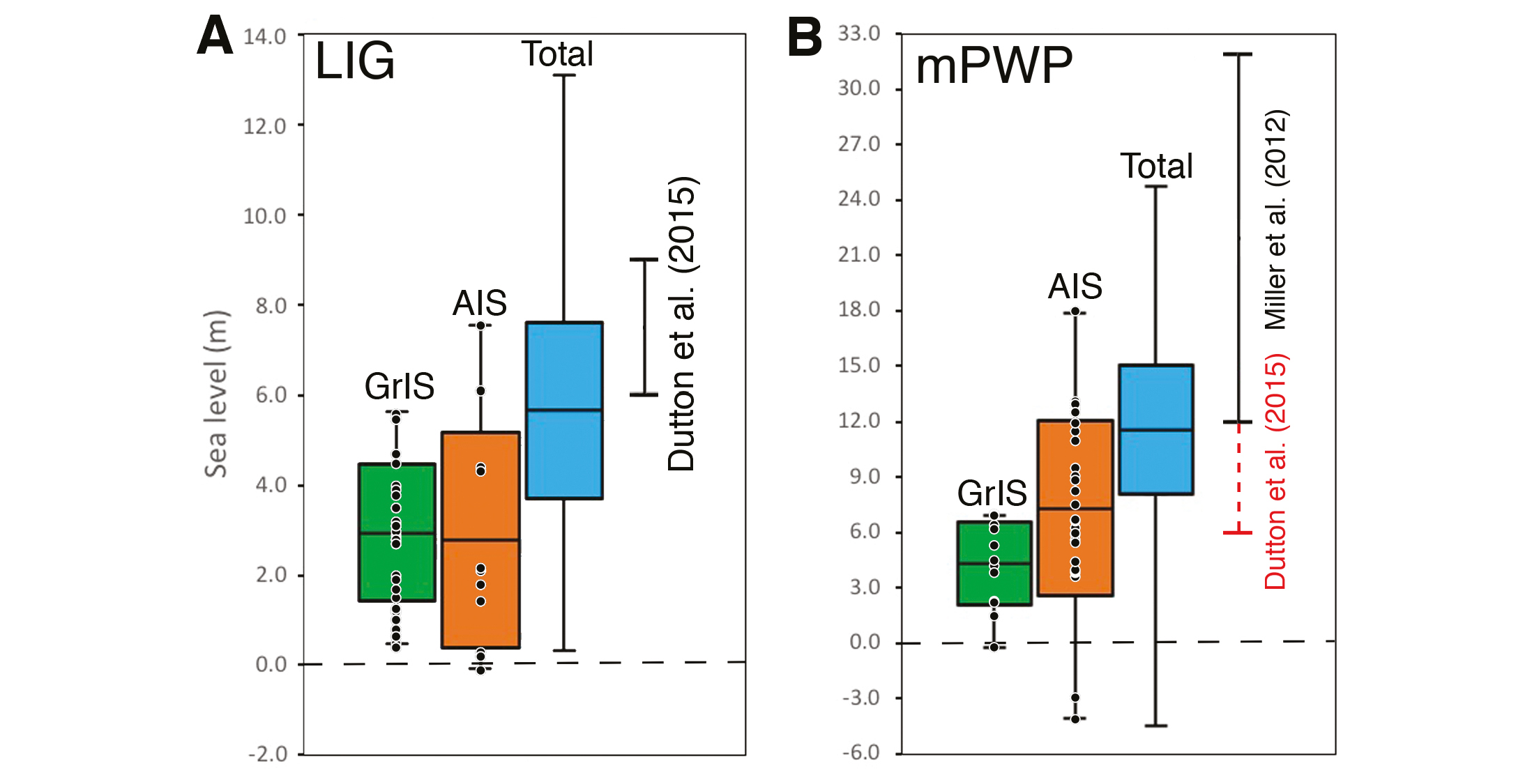
Over recent decades, numerous studies have estimated the contribution to past sea level from the GrIS and AIS (Fig. 2). Different approaches have been used, using either a single surface-air temperature anomaly or steady state climate forcing, transient or equilibrium simulations, or fully coupled to a (lower resolution) climate model (see for example overviews in Dutton et al. 2015; Dolan et al. 2018; Plach et al. 2018). The broad range of simulated individual contributions from the GrIS and AIS clearly illustrate the uncertainties related to the use of different ice-sheet and climate models to estimate past sea-level changes (as also shown in Dolan et al. 2018).

Figure 2: Overview of published sea-level contributions (in meters) from the GrIS (green) and AIS (orange). (A) The LIG compared with the range from Dutton et al. (2015) and (B) the mPWP compared with the range from Dutton et al. (2015) in red, and Miller et al. (2012) in black. Simulations are shown by the black dots in (A) and (B); sources are listed in the online supplementary material. From each source we used either one value or the mean value of an ensemble, including the range. Boxes indicate the total mean, with one standard deviation. The maximum and minimum modeled ice sheet within the total ensemble are indicated by the whiskers (in black). Totals (blue) are calculated by summing the mean, minimum and maximum and averaging the standard deviations from the GrIS and AIS. References listed below.

The total mean sea-level change estimated from ice-sheet models is on the low end compared to the geological evidence for both the LIG and the mPWP (blue boxes in Fig. 2a,b). A higher contribution from the LIG AIS could stem from interactions with the ocean (e.g. Sutter et al. 2016), although two-way interaction with the climate cannot be ignored. The driving processes leading to increased ice-cliff calving are not yet fully understood but could account for a significant retreat of the LIG and mPWP AIS (DeConto and Pollard 2016), whereas gaps in knowledge of the subglacial topography leads to greater uncertainties for AIS contribution to mPWP sea level (Gasson et al. 2015). Surface melt of the GrIS can be significantly enhanced relative to the present due to increased summer insolation (Fig. 1c,d) during the mPWP and LIG (Robinson and Goelzer 2014; de Boer et al. 2017).

Outlook

Precisely quantifying the impact of processes, such as calving and ice-cliff failure, on the GrIS or AIS and the impact of the interaction between ocean warming and sub-glacial topography on ice-sheet retreat remains challenging (DeConto and Pollard 2016). Nonetheless, more precisely located and time-varying geological data will allow for a much more detailed study of coupled paleo ice-sheet climate simulations. This might reduce model-data discrepancies and lead to a consensus of past sea-level contributions from the GrIS and AIS in the coming years, thus providing stronger constraints to future sea-level projections.

affiliations

1Faculty of Science, Earth and Climate, Vrije Universiteit Amsterdam, The Netherlands
2National Institute of Oceanography and Experimental Geophysics, Trieste, Italy
3Antarctic Research Centre, Victoria University of Wellington, New Zealand
4Department of Geoscience, University of Massachusetts Amherst, USA

contact

Bas de Boer: bas.de.boer@vu.nl

references

Colleoni F et al. (2018) Nat Commun 9:2289

Dolan AM et al. (2018) Nat Commun 9:2799

de Boer B et al. (2017) Geophys Res Lett 44: 10,486-10,494

DeConto RM, Pollard D (2016) Nature 531: 591-597

Dutton A et al. (2015) Science 349: aaa4019

Huybrechts P (2002) Quat Sci Rev 21: 203-231

Gasson et al. (2015) Geophys Res Lett 42: 5372-5377

Golledge NR et al. (2017) Geophys Res Lett 44: 2343-2351

Laskar J et al. (2004) Astron Astroph 428: 261-285