By: Sicard M, de Boer AM & Sime LC
Available in: Past Global Changes Magazine 30(2), 92-93, 2022
> Access contents of this issue
> Download this article as pdf
The 16 models that simulated the Last Interglacial climate as part of the CMIP6/PMIP4 exercise consistently produce a smaller Arctic summer sea-ice area compared to the pre-industrial period, but their reduction ranges widely (28–96% of the pre-industrial area). Causes for these differences need further investigation.
Why are we interested in changes in the Arctic sea ice during the Last Interglacial?
The Last Interglacial (LIG, 129-116 kyr before present (BP)) is characterized by a strong insolation forcing leading to an Arctic land summer warming of 4–5°C relative to the pre-industrial period (PI; Guarino et al. 2020). The increase in surface temperatures has been associated with changes in Arctic sea ice potentially comparable in magnitude to those projected for the near future (Guarino et al. 2020). Simulations of the LIG climate, thus, provide a tool to study the processes and feedbacks related to current Arctic sea-ice loss and polar warming. The high availability of sea-ice proxy data, compared to previous interglacial periods, also makes the LIG a good case study to evaluate the ability of climate models to simulate sea ice during periods warmer than today. In recognition of the importance of the LIG in our understanding of climate change, it was formally included as a target period in the latest Paleoclimate Modelling Intercomparison Project (PMIP4). The joint experimental protocol differs primarily from the PI experiment in the astronomical parameters and greenhouse gas concentrations (Otto-Bliesner et al. 2017). The LIG PMIP4 experiment, thus, represents a reference point for discussions of model reconstruction of Arctic sea ice for this period.
What have we learned from the CMIP6/PMIP4 LIG experiment?
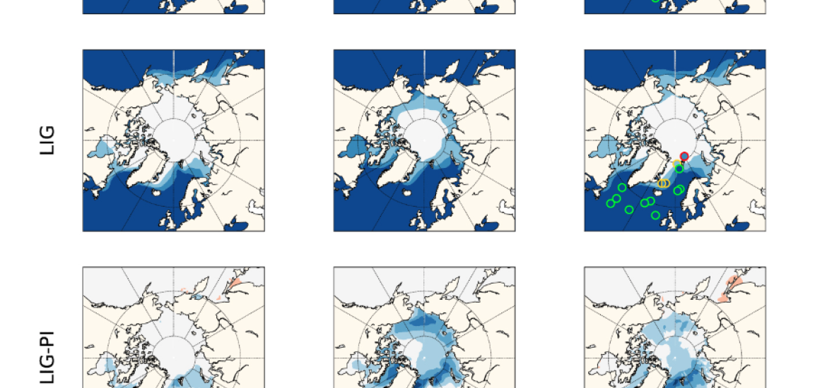
The Arctic sea ice, simulated by the 16 climate models that run the LIG experiment, was analyzed by Kageyama et al. (2021). Figure 1 shows the multi-model mean (MMM) for the winter (DJF), summer (JJA) and annual sea-ice concentration. The larger sea-ice retreat relative to the PI appears in summer when the insolation anomaly reaches its maximum. During this season, the Greenland, Barents and Chukchi seas experience the most significant ice loss. The minimum monthly MMM at the LIG is equal to 3.2 ± 1.5 × 10⁶ km2, which represents a decrease of about 50% compared to the PI. Three models (HadGEM3-GC3.1-LL, CESM2, and NESM3) simulate an above-average retreat of the sea-ice edge in summer relative to the PI, with a total sea-ice area close to, or less than, 1 × 10⁶ km2. However, of these three, only HadGEM3-GC3.1-LL and CESM2 have a realistic representation of the PI Arctic sea-ice seasonal cycle. The HadGEM3-GC3.1-LL model shows the largest sea-ice retreat, with the Arctic Ocean becoming ice-free at the end of summer (Guarino et al. 2020). On the other end of the spectrum, the INM-CM4-8, GISS-E2-1-G and FGOALS-g3 models simulate large sea-ice areas greater than 5 × 10⁶ km2 at the end of summer. This disparity between models is also found in winter. During this season, the maximum monthly MMM is equal to 16.0 ± 2.6 × 10⁶ km2, with most models simulating a slight increase compared to the PI. However, the ACCESS-ESM1-5, EC-Earth3-LR and INM-CM4-8 models show a reduced sea-ice area relative to the PI.
What is the cause of inter-model differences?
There are many characteristics of climate models that can lead to variable results, including differences in model physics and chemistry, discretization scheme and numerical resolution, parameterization of subgrid-scale processes, and tuning parameters.
> Continue reading ...
Figure 1: Multi-model mean of the Arctic sea-ice concentration for the pre-industrial (PI) and Last Interglacial (LIG) periods and LIG-PI differences. Results are plotted for winter (DJF), summer (JJA) and the annual average. The fill color of the symbols corresponds to the observed values at sites where proxy data are available for the LIG (see Kageyama et al. (2021) for more details on the sea-ice data synthesis). For the PI, a dataset obtained from different satellite and in-situ observations is used (Reynolds et al. 2002). The color of the symbol outline indicates the number of models simulating the observed sea-ice cover: green for nine or more models, yellow for five to nine models and red for five or fewer models. Adapted from Kageyama et al. (2021).
Available in: Past Global Changes Magazine 30(2), 92-93, 2022
> Access contents of this issue
> Download this article as pdf