PAGES Magazine articles

The poor preservation potential of tsunami records in arid environments has prevented detailed studies of tsunami-washed sand deposits along these coasts. However, recent studies have shown that evidence of these high-energy marine events is camouflaged within (hyper)arid landscapes.

In general, the study of recent paleotsunamis has been based on the identification and analysis of their onshore deposits, in the absence of historical or archaeological evidence (e.g. Engel et al. 2020; Prizomwala et al. 2024). High-energy waves mix the marine sediments they drag from the seabed with the continental deposits they flood, resulting in a layer of sand containing a melting pot of grains and microfossil remains.

Scientists studying paleotsunamis look for areas where these sediments are trapped and, in most cases, they find them in very similar environmental scenarios: coastal wetlands and lagoons near river mouths, or even continental lakes near the shoreline where waves can reach and deposit the sediment they transport.

The presence of large bodies of freshwater is a common characteristic, as it favors the accumulation of the tsunami deposits. In addition, the subsequent, and continuous sedimentary dynamics buries them, allowing their preservation in the sedimentary record. But, what happens when a tsunami impacts coasts where these freshwater bodies do not exist, such as in the Atacama Desert in Chile, the driest place in the world? Without wetlands, lagoons, estuaries, or deltas, how are the tsunami deposits preserved?

Why study the tsunami record of the southern Atacama Desert?

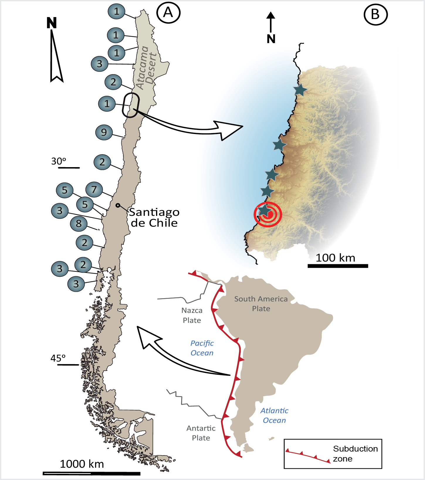
The Chilean coast is a highly seismic and tsunami-prone hazard zone, owing to the convergent boundary where the Nazca Plate subducts below the South American Plate (Fig. 1). In this setting, tens of earthquakes with focal mechanisms and magnitudes large enough to trigger highly destructive tsunamis must have been generated during the Late Holocene, although no great earthquakes (moment magnitude [Mw] ≥8.6; Klein et al. 2017) have been reported in the historical chronicles of the southern edge of the Atacama Desert (Fig. 1). In fact, only two large-magnitude earthquakes that triggered destructive tsunamis occurred in historic times; in 1819 and 1922 CE (Ruiz and Madariaga 2018).

There is still great uncertainty regarding the number and magnitude of large paleotsunami events in this sector of the Atacama Desert during the Late Quaternary, caused by the challenging accessibility and long distances from major cities that have prevented exploration of these coasts. The less-evident record of tsunami deposits linked to environmental constraints when compared with other zones of Chile contributes to this uncertainty (Fig. 1).

Figure 1: (A) Location of the places where records of paleotsunamis have been described on the coast of Chile. The number inside the colored circle indicates the number of works carried out on this topic (based on León et al. 2022). (B) Detail of the southern Atacama Desert coast. Stars indicate potential sites for tsunami research and the red circle indicates the epicenter of the 1922 CE Atacama earthquake.

The tsunami record on arid coasts: Boulder deposits

On arid, rocky coasts, such as those of northern Chile, tsunamis are not commonly recorded as sand layers interbedded with finer sediments, but as boulder fields on top of cliffs. Some of these reach weights of hundreds of tons and were moved from areas located up to 10 m above sea level (Abad et al. 2020). These deposits form when the tsunami waves impact the rocky cliff, detach a boulder, creating a boulder niche, and transport it landwards tens to hundreds of meters. The orientation of the boulders can be used to interpret the wave direction, and their size and mass can be used to model the scale of the extreme waves and their flow velocities. The advantage of these deposits is that they cannot be reworked by the wind after their deposition; thus, they provide exceptional tsunami evidence on arid coasts that prevail in the landscape without being practically modified over time. Unfortunately, the scenario in which this type of evidence is formed is very specific, and the recording of events through these records is very incomplete. In some cases, a boulder field can even be the result of successive large tsunamis.

The tsunami record on arid coasts: Fine grained deposits

In the absence of cliffs and freshwater bodies that may preserve the large volumes of sand brought from the sea to the coasts of the Atacama Desert, the sediments are deposited on vast coastal plains and become part of the dune fields, which bear little resemblance to the classic description of "tsunamiites" in scientific literature (Shiki and Yamazaki 2008). The apparent absence of this geological evidence should not be interpreted as evidence of its absence. This is perhaps one of the last challenges that remains to be overcome in tsunami science, and it must be addressed from a holistic perspective, in order to determine the tsunamigenic origin of camouflaged morphogenic and sedimentary evidence.

So, where, and how, do we look for "classic" and probably clearer evidence of paleotsunami(s) in the Atacama Desert? Along thousands of kilometers of arid coast there are a few exceptional places in which a combination of geomorphological, climatic and geological factors exist, and small coastal wetlands have been formed, owing to the emergence of groundwater in the permanent absence of surface waters that reach the sea. Nevertheless, the probability of marine high-energy events being recorded and preserved in these environments is low, because several processes may alter them.

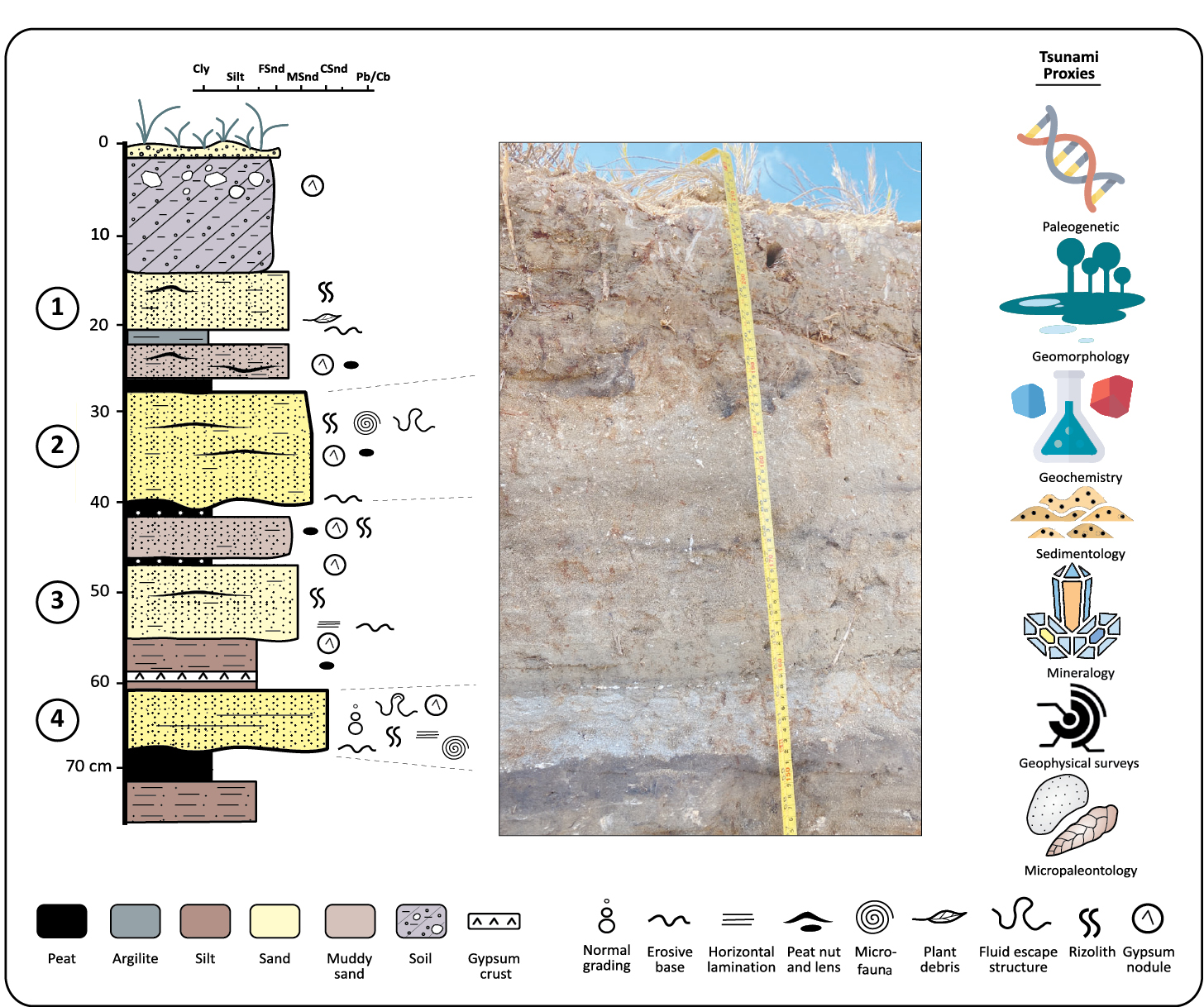
Figure 2: Detailed sedimentological section elaborated in an arid coastal wetland in the southern Atacama Desert. Numbers indicate sand layers of a distinctive lighter color formed by tsunamis. The formation of saline crusts and gypsum nodules, as well as the burrowing of roots, usually mask these records.

Firstly, after the marine flooding occurs and seawater retreats, evaporation of the wet marine sediments begins. This newly deposited material includes sea salts that precipitate, as evaporation continues, forming saline crusts and nodules that will mask the tsunami deposit in the geological record (Fig. 2). In fact, tsunami sand or mud deposits can be misinterpreted as paleosoils in the field. If this salt precipitation process does not occur, the absence of sedimentation in arid environments will not protect them from eolian processes, leading to an incomplete tsunami record.

Finally, ephemeral rivers, where coastal wetlands are formed, are occasionally activated when intense El Niño-Southern Oscillation-related rain occurs in the desert. These continental flows present a strong erosive capacity, even near the river mouth, and can dramatically change the coastal wetland configuration, as occurred after the March 2015 CE rains in Atacama (Abad et al. 2017).

A multi-proxy solution

The solution to these issues is neither simple nor straightforward. Only a few sectors of the Atacama Desert coastal segment seem to fulfill the geomorphic requirements, and even at those locations, a multi-proxy detailed study is needed to untangle the paleotsunami record of the last 4000 years. At these locations, each layer, generally less than 10 cm thick, must be sampled and subjected to a variety of analyses looking for the proxy or their combination, which allows us to classify the deposit as sediments formed by a tsunami.

At temperate latitudes, the combination of grain size and micropaleontology or geochemistry is normally sufficient to claim a deposit as a tsunami layer. However, on these arid coasts, grain size may have been modified by eolian rework, microfauna may have been dissolved, and the geochemistry of the sediment may have been altered by later precipitation of gypsum. Thus, we will have an answer only if we consider a more holistic solution. Geomorphological and sedimentological analyses are still key, but they must be combined not only with microfossil and geochemical analyses, but also with mineralogical, geophysical and even environmental DNA analysis to be sure that this sand layer was formed by a paleotsunami (Fig. 2). The effort to unmask this evidence is enormous, and requires the participation of multidisciplinary teams formed by geologists, paleontologists, biologists, and geophysicists, without whom it would be impossible to achieve the ultimate goal of assessing the tsunami hazard to which the southern Atacama coast is exposed.

To date, the low number of tsunami studies on arid coasts has not only led to a misunderstanding of the tsunami events on these coasts compared to temperate and humid areas, but also to underestimating the risk that coastal communities are exposed to by ignoring the recurrence of these high-energy marine events and their magnitude throughout the geological record. Until we understand them, we will continue to search for sand in the desert.

ACKNOWLEDGEMENTS

This article reviews the challenges addressed by the research project TRAMPA: grant PID2021-127268NB-100 funded by MCIN/AEI/ 10.13039/501100011033 and by "ERDF A way of making Europe", by the EU.

affiliationS

1Department of Biology and Geology, Physics and Inorganic Chemistry, Rey Juan Carlos University, Madrid, Spain

2Research Group in Earth Dynamics and Landscape Evolution, Rey Juan Carlos University, Madrid, Spain

contact

Tatiana Izquierdo: tatiana.izquierdo@urjc.es

references

Abad M et al. (2017) Geomorphic effects and sedimentological record of flash floods in the Copiapó River salt marsh (Atacama coast, Northern Chile). EGU 2017 General Assembly Conference, Vienna, Austria

Abad M et al. (2020) Sedimentology 67(3): 1505-1528

Engel M et al. (2020) In: Engel M et al. (Eds) Geological Records of Tsunamis and Other Extreme Waves (First Edition). Elsevier, 3-20

Klein E et al. (2017) Earth Planet Sci Lett 469: 123-134

Prizomwala SP et al. (2024) PAGES Mag 32(1): 36-37

Ruiz S, Madariaga R (2018) Tectonophysics 733: 37-56

Shiki T, Yamazaki T (2008) In: Shiki T et al. (Eds) Tsunamiites (Second Edition). Elsevier, 5-7

A study of tsunami deposits preserved in coastal sedimentary sequences of southern Peru suggests that five very large tsunamigenic earthquakes with moment magnitude (Mw) >8.5 occurred during the last 2500 years, including the 1604 and 1868 CE tsunamis.

Timescales of tsunami and earthquake record

Subduction-zone megathrust faults cause the largest earthquakes on Earth. The recent megathrust earthquakes in 2004 in Sumatra (Indonesia; Mw 9.3) and 2011 in Tōhoku-oki (Japan; Mw 9.1), and their associated tsunamis, highlighted a weakness in the integration of the time factor in hazard evaluation. Indeed, tsunami-hazard evaluation must combine both historical evidence of tsunamis (recorded or observed events) and geological evidence (tsunami deposits). This is particularly critical when the historical catalogs are limited in time, and/or when the largest events have a long period of return, thus being potentially absent from the historical record.

In Peru, the time period covered by the catalogs of earthquakes and associated tsunamis is limited to the last five centuries, with the oldest event dating back to 1582 CE (Comte and Pardo 1991; Dorbath et al. 1990). Time acts as a filter, and very few earthquakes of Mw <7.5 are mentioned in the archives before the 19th century (Kulikov et al. 2005). Paleotsunami studies have the potential to enlarge the timescale of tsunami catalogs up to the early Holocene. This represents a crucial contribution to the assessment of earthquake and tsunami hazards.

Historical tsunamis in southern Peru

In Peru, based on statistics of historical events, the return periods of Mw ~8 and Mw ≥8.7 tsunamigenic earthquakes are estimated at 10 and 100 years, respectively (Kulikov et al. 2005). A total of 10 tsunamigenic earthquakes have occurred in southern Peru (south of Nazca Ridge) since 1530 CE (Comte and Pardo 1991; Dorbath et al. 1990; Okal et al. 2002), including five major events in 1604 (Mw 8.7, with a tsunami up to 16 m high when arriving on shore), 1687 (Mw 8.4, 10 m), 1784 (Mw 8.4, 4 m), 1868 (Mw 8.8, 18 m), and 2001 CE (Mw 8.4, 8.8 m). Regional earthquakes in central Peru (1687, 1746 and 2007 CE) and northern Chile (1615, 1877 and 2014 CE) also generated tsunamis that were observed on the coasts of southern Peru. Trans-Pacific tsunamis caused by far-field sources (Japan, Tonga, etc.) typically produce wave heights lower than 3 m on the coast of Peru.

Additionally, Spiske et al. (2013a) found two tsunami deposits dated 615 BCE–119 CE, and 207 BCE–255 CE, which represent the only evidence of paleotsunamis published so far in southern Peru. Abad et al. (2020) described a coastal boulder-field dated between the 13th and 16th centuries.

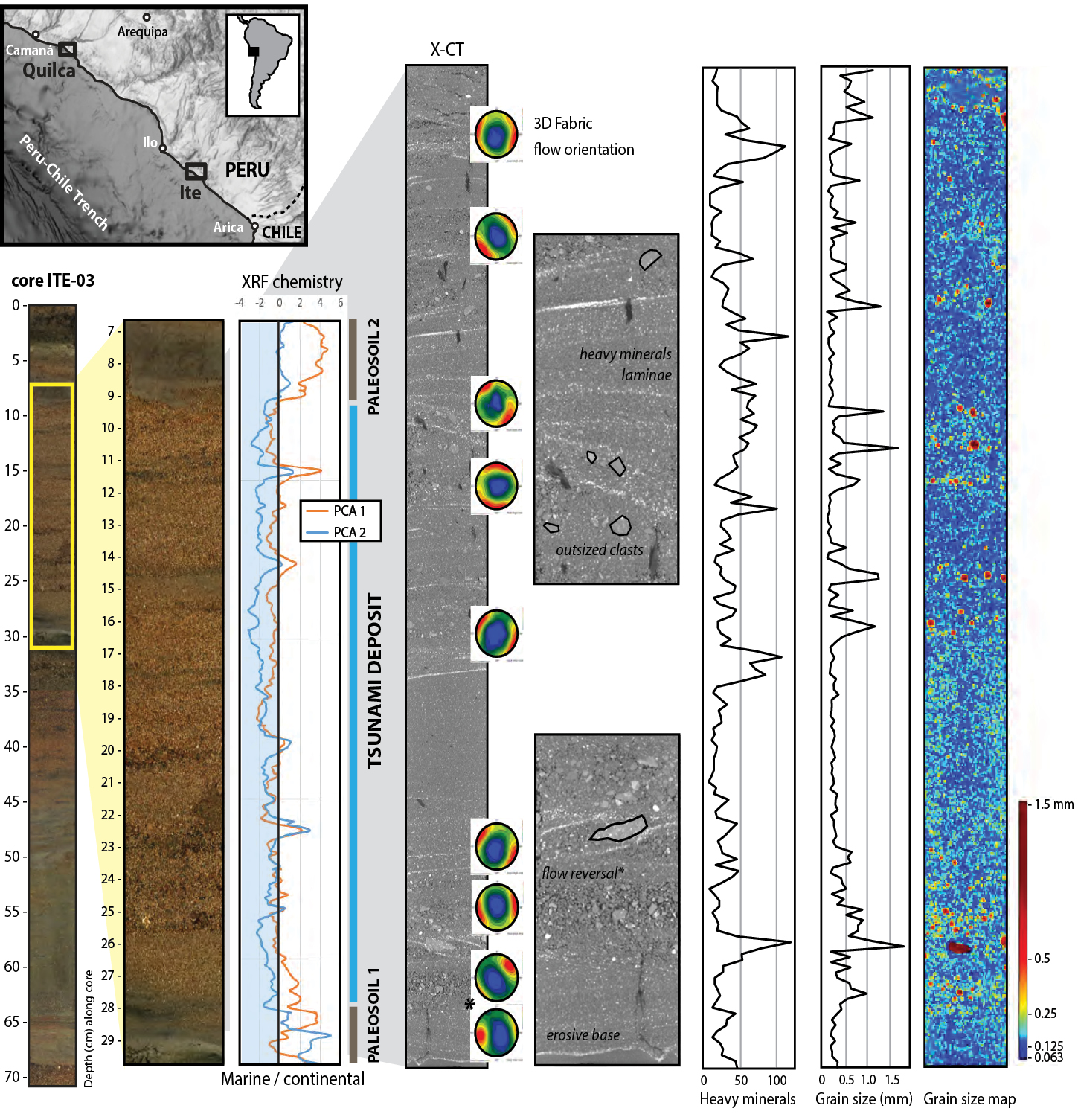
Figure 1:  Location of the study sites in southern Peru, and methods used to identify tsunami deposits in the coastal sedimentary record. (A) Photography of the core. (B) Close-up view of a tsunami deposit. (C) Principal Component Analysis (PCA) of XRF core-scanner data. (D) X-CT (X-ray computed tomography). (E) Stereograms of sedimentary fabric. (F) Abundance of heavy minerals. (G) Grain-size data inferred from X-CT.

Paleotsunami sites and methods

In this study we investigated two coastal sites in southern Peru: the Ite lagoon (south of Ilo) and the Quilca floodplain (south of Camana) (Fig. 1). Samples were collected along trenches, using both U-channels and push cores, as well as bulk samples of available sediments. Laboratory analyses consist of combining XRF core-scanner, SEM (Scanning Electron Microscope), X-ray computed tomography (X-CT), and DNA metabarcoding methods to characterize the structure, grain size, fabric, chemical, mineralogical, and biological compositions of the sediments. This workflow was previously applied to storm and tsunami deposits, as explained in Sabatier et al. (2010), Cuven et al. (2013), Paris et al. (2020) and Biguenet et al. (2022).

We also tested a DNA approach: samples of tsunami and terrestrial deposits were directly collected from the field with sterile devices, immediately dessicated for preservation and processed following the methodology by Bremond et al. (2017), specifically targeting 18S rDNA region V7 (a region of nuclear DNA encoding 18S nuclear ribosomal RNA, as commonly used for eukariotes in metabarcoding: Guardiola et al. 2016). Samples of wood fragments and organic sediment were 14C dated at Laboratoire de Mesure du Carbone in France using accelerator mass spectrometry (Dumoulin et al. 2017).

A 2500-year chronology of tsunami deposits

Tsunami deposits identified in the sedimentary sequences appear as fine-to-medium sand units intercalated in dark-brown lagoonal mud at Ite, or brownish overflow silt at Quilca. These sand units are characterized by an increased marine signature compared to background sediments, as evidenced by vertical variations of the chemical composition (Fig. 1). Grain-size distribution shows that the sand units have a variable proportion of silt and clay, which reflects the mixing of different sediment sources. The sand is made of silicate minerals (quartz being dominant), with some oxides, as well as wood, plants, and sparse marine bioclasts (foraminifera, small fragments of shells). DNA analyses record a mixed marine-continental composition, especially in Quilca where DNA show marine algae, ciliates and worms, Pacific coral reef fish, along with brakish diatom species, Andean plants, and terrestrial ciliates and worms.

The base of the sand units is often erosive, thus forming rip-up clasts of mud or soil inside the sand. Their internal structure is emphasized by horizontal to low-angle bedding, heavy-minerals laminae, erosive discontinuities between subunits, and vertical variations of the grain size (including clast-supported lenses of coarse sand, and matrix-supported silt-rich subunits). Different types of sedimentary fabric were inferred from X-CT: flow-parallel fabric oriented landward (wave uprush) or seaward (flow-reversal or backwash), and flow-transverse fabric (Fig. 1).

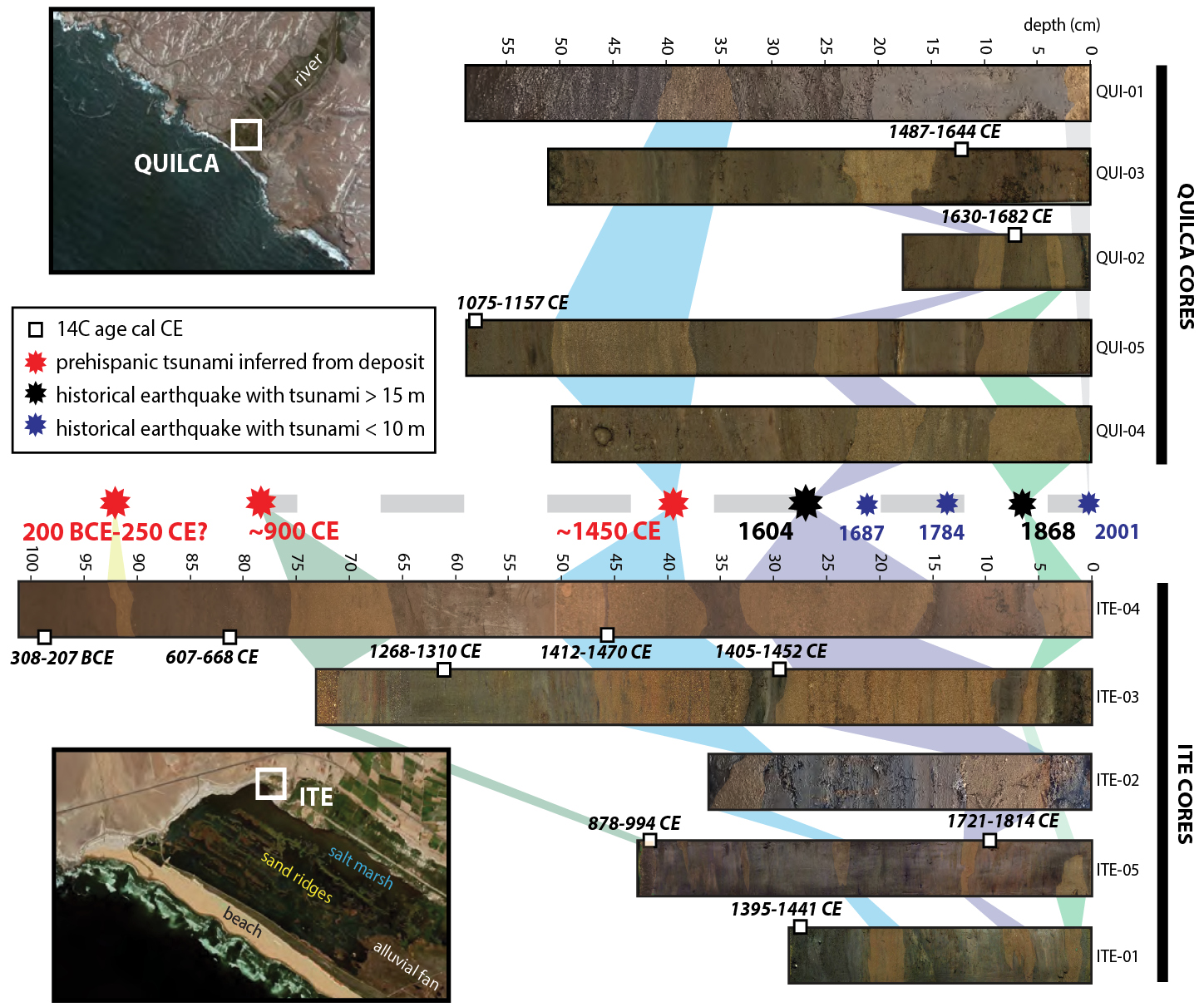
The sedimentary sequences (and thus the tsunami chronology) are time-constrained by 14C ages that range between 308–207 BCE (100 cm depth) to 1721–1814 CE (10 cm depth) at Ite, and 1075–1157 CE (60 cm depth) to 1630–1682 CE (7 cm depth) at Quilca (Fig. 2). The 1604 and 1868 CE tsunamis are well recorded at both sites. The 1604 CE tsunami deposit is particularly thick (up to 20 cm) at Ite. We also found three prehispanic tsunamis. A major tsunami at ~1450 CE is preserved at both sites. Two older tsunamis are found at Ite: one at ~900 CE, and the oldest one between 200 BCE and 250 CE (which could correspond to the 207 BCE–255 CE event of Spiske et al. 2013a).

Figure 2: Location of the core samples in Quilca and Ite, and synthetic extended chronology of tsunami events in Southern Peru.

Earthquake magnitude versus tsunami-deposit preservation

In southern Peru, the last five major earthquakes (Mw ≥8.4) occurred at quite regular intervals (every 83–133 years), but there is a variability in the rupture extent (Dorbath et al. 1990; Philibosian and Meltzner 2020). The more extensive ruptures occurred in 1604 and 1868 CE, which is concordant with the tsunami-deposit records. Indeed, historical tsunamis with wave heights >15 m, such as the 1604 and 1868 CE ones, are well recorded in the coastal stratigraphy (tsunami deposits being typically 5–20 cm thick), whereas tsunamis with wave heights <10 m in the study area (e.g. 1687, 1784 and 1877 CE) are apparently not preserved in lagoons that are protected by coastal sand ridges.

As an example, the 2001 CE tsunami had wave heights up to 2.3 m in Quilca (Okal et al. 2002). During our field survey in 2017, traces of the 2001 CE tsunami were still visible in the form of irregular and sparse sand layers (up to 1.5 cm thick at 100 m from the shoreline, but 420 m away from the riverbed), abundant drift wood, and anthropic debris. Spiske et al. (2013b) reported a decrease of the average thickness of the 2001 CE tsunami deposits from 0.5–28 cm to 0.1–6 cm in only six years, and concluded that even in such an arid environment, the sedimentary record of tsunamis may not fully represent a comprehensive tsunami hazard.

Thus, there seems to be a threshold of earthquake magnitude (Mw >8.5 in southern Peru) to generate a tsunami large enough to be preserved in the sedimentary record. Our study reveals that only five very large earthquakes left tsunami deposits in coastal lagoons of southern Peru during the last 2500 years, while 10 tsunamis occurred during the last 500 years.

ACKNOWLEDGEMENTS

Grant IRD and Labex OSUG@2020 (ANR10 LABX56). CNRS-INSU ARTEMIS Radiocarbon AMS at LMC14. A.L. Develle and P. Sabatier (EDYTEM Chambéry ), E. Ando and P. Charrier (3SR Grenoble). ClerVolc contribution n° 636.

affiliationS

1Mercator Ocean International, Toulouse, France

2Université Clermont Auvergne, CNRS, IRD, OPGC, Laboratoire Magmas et Volcans, Clermont-Ferrand, France

3IRD, Université Grenoble Alpes, CNRS, ISTerre, Grenoble, France

4Laboratoire d’ÉCologie Alpine, Université Grenoble Alpes, CNRS, LECA, Grenoble, France

5INGEMMET, Lima, Peru

contact

Raphaël Paris: raphael.paris@uca.fr

references

Abad M et al. (2020) Sediment 67: 1505-1528

Biguenet M et al. (2022) Mar Geol 450: 106864

Bremond L et al. (2017) Quat Sci Rev 170: 203-211

Comte D, Pardo M (1991) Nat Haz 4: 23-44

Cuven S et al. (2013) Mar Geol 337: 98-111

Dorbath L et al. (1990) Bull Seism Soc Am 80: 551-576

Dumoulin J-P et al. (2017) Radiocarbon 59: 713-726

Guardiola M et al. (2016) Plos One 11(4): e0153836

Kulikov EA et al. (2005) Nat Haz 35: 185-209

Okal EA et al. (2002) Seismol Res Lett 73: 904-917

Paris R et al. (2020) Sediment 67: 1207-1229

Philibosian B, Meltzner AJ (2020) Quat Sci Rev 241: 1066390

Sabatier P et al. (2010) Sed Geol 228: 205-217

Spiske M et al. (2013a) Quat Int 305: 31-44

Spiske M et al. (2013b) Earth-Sci Rev 126: 58-73

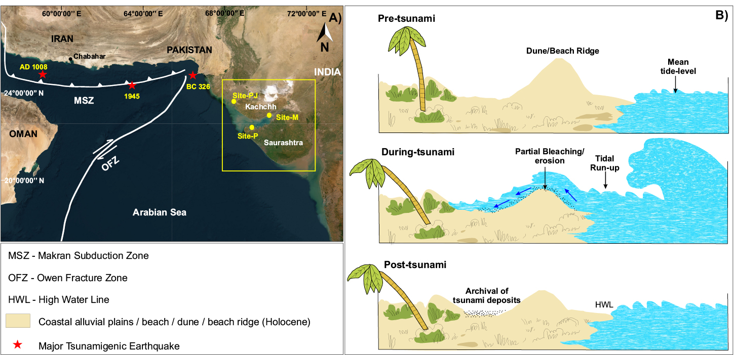
Sedimentary deposits bearing potential paleotsunamis and/or cyclonic-storm records were studied along the western shoreline of India using a multi-proxy approach, as this helps to better assess the source of the wave(s).

The northern Arabian Sea hosts a major tsunamigenic source, i.e. the Makran Subduction Zone (MSZ), which has produced instrumental, historical and paleo-period tsunami waves that have caused damage on the shorelines of western India, Pakistan, Iran, and Oman (Fig. 1a). However, the shoreline of western India in this context has remained unexplored. The western coast of India, owing to its varied geomorphology (rocky coastline to sandy beaches/mudflats) has been impacted by past tsunamis; those footprints are preserved in the form of boulder blocks to sand sheets deposited far inland from the present-day shoreline (Bhatt et al. 2016; Prizomwala et al. 2015, 2018, 2021, 2022). Although the recurrence and larger catalog for the Holocene period are yet to be completed, the evidence of several major tsunamis generated by MSZ has been discussed briefly in recent literature (Prizomwala et al. 2021).

One problem in the study of sandy onshore deposits is that tsunamis are difficult to distinguish from storm deposits (Gouramanis et al. 2024; Yap et al. 2021). However, a combination of multi-proxy techniques can help to better assess the origin of the wave(s) that lead to the sedimentary deposit in question. This paper highlights the use of multi-proxy records in sand deposits to distinguish tsunamigenic sources from other coastal processes, most notably the cyclonic storms, on the western Indian shoreline. The coastlines of Kachchh and southwestern Saurashtra show beach-ridge dune-type assemblages suitable for preserving signatures of such events. Thus, they were used as study sites for the investigation of past extreme events (Fig. 1b).

Figure 1: (A) Tectonic setup of the northern Arabian Sea with tsunamigenic sources. (B) Schematic scenario for a pre-, during- and post-tsunami event, along a with beach-ridge-dune configuration.

Tsunami and storm deposits: Process, source, and character

Tsunamis can erode the seabed due to their high energy, and transport the eroded sediment in suspension onshore (supratidal regime). While receding after the maximum inundation, a significant part of the sediment/debris load is often deposited, while a minor part is transported offshore (Fig. 1b). Apart from tsunami waves, cyclonic storm surges also possess a similar character; however, they are of relatively lower intensity compared to tsunami waves. Storm surges are also often known to erode the seabed, but at relatively shallower depths (<10–20 m). Hence, the sedimentary deposits of a tsunami differ from a storm, or other coastal process-derived deposits, by 1) their inland extent; 2) the presence of deeper sediment and fauna; and 3) the chaotic nature of the deposits (debris filled, lack of sorting) (Chagué-Goff et al. 2011; Dawson and Stewart 2007; Kortekaas and Dawson 2007; Morton et al. 2007; Prizomwala et al. 2018). However, several storms (e.g. Typhoon Haiyan in 2013) deposited sediments with similar characteristics to those from tsunamis, making them more challenging to distinguish (Soria et al. 2017). Therefore, it is crucial to assess the recorded (instrumental) storm history of a region together with a probable worst-case scenario (most intense storm and its characteristics), while comparing and assessing a probable tsunami-deposit inference.

Multi-proxy record of sedimentary deposits from the western coastline of India

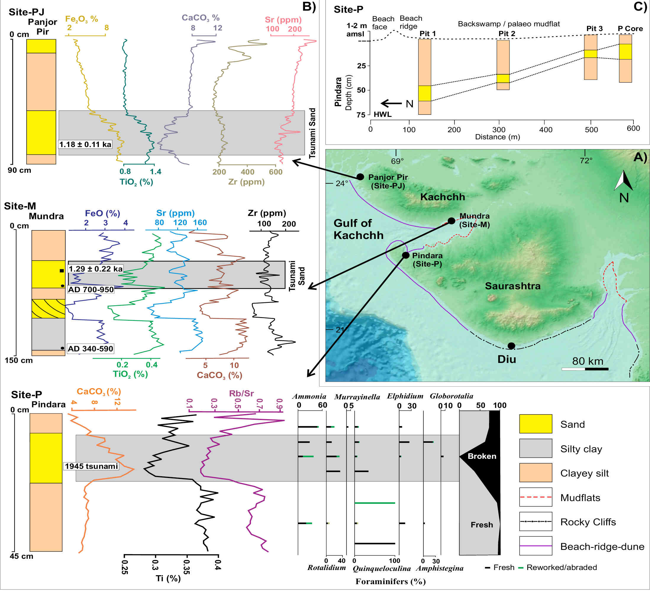
Sediment geochemical proxies can be very reliable for discriminating different source signals, particularly when there is a mixing of tsunami-derived sand and local processes (Chagué-Goff 2010; Prizomwala et al. 2018, 2022; Srinivasalu et al. 2008). For example, the sand derived from shallower offshore sand shoals in the Gulf of Kachchh off the Pindara (site-P) and Kachchh (site-M) coastline comes from the Deccan Basalts (Fig. 2a). These sediments are richer in Fe2O3, TiO2, Zr and Sr, owing to their provenance from the Deccan Basalts (see Prizomwala et al. 2018 for details). Their higher concentration in CaCO3 is due to the high content of broken shells and foraminifera in sandy sediments, which are likely derived from offshore erosion. Previous researchers have inferred that these sands were eroded during historically known tsunami events, such as the 1945 CE tsunami event and the 1008 CE event along the MSZ, and deposited in the form of a sand layer at the Pindara (site-P) and Kachchh (site-PJ & M) coastlines (Prizomwala et al. 2018, 2022). The geochemical signatures are a useful tool for linking offshore geological provenance to the sand layer deposited inland, owing to the extreme event. For the Kachchh coast in particular, the sediments from the Deccan Basalts overwhelms the signature in inferred tsunami sand horizons.

Figure 2: (A) Inset shaded relief map of Gujarat (western India). (B) Temporal geochemical and foraminiferal distribution of sedimentary deposits at sites P, PJ and M. (C) An onshore extent of tsunami sand layer with across-coast profile of site-P

The onshore (landward) extent of sedimentary deposits is one of the most common approaches for distinguishing a tsunami deposit from a probable storm surge deposit (Kortekaas and Dawson 2007; Morton et al. 2007; Prizomwala et al. 2018, 2022). The coastal remnants of the deposits along the Pindara (site-P) coast are observed in the form of sand sheets, reaching up to 580 m inland from the high-water line (HWL) (Fig. 2b). The sand-sheet geometry was probed using multiple shallow pits across the coast. Available records of the most intense storms in the Arabian Sea show a much more limited spatial extent in their inland sediment transport deposit (Prizomwala et al. 2018).

The sedimentological signature of these tsunamis is characterized by the lack of sorted grains, with overall landward fining along with the presence of mud intraclasts, broken shell and foraminifera. These observations demonstrate the high-energy wave character, which essentially eroded the bottom of the offshore seabed (Kortekaas and Dawson 2007; Morton et al. 2007; Shanmugam 2012). Storms, on the other hand, exhibit a comparably better sorting, the absence of mud-intraclasts and the presence of several sedimentary structures. The increase in benthic foraminiferal diversity, and the presence of species occurring offshore, consolidates the assumption of the tsunami origin of these sand layers (Chagué-Goff et al. 2011; Prizomwala et al. 2022).

Outlook

The debate regarding the differentiation of sedimentary deposits from tsunami and cyclonic storm surges from the Arabian Sea requires an investigation of more modern analogues (e.g. Gonu, the only super cyclone in the instrumental history of the Arabian Sea, which occurred in 2007). There is a need to study more of these past tsunamigenic events from the Arabian Sea in order to build a catalog spanning at least the Holocene period. Similarly, compared to tsunamis, the available data of storms is extremely limited and needs to be augmented using geological records. More robust and complete information regarding the extent, type and nature of super cyclonic storm-surge deposits would help to assess the threshold for differentiating both wave types. Such information is a prerequisite for a better coastal hazard assessment, which is crucial for the safety of the fast-developing coastal infrastructure. A multi-proxy approach involving sedimentology, geochemistry, micropaleontology, and the landward extent of the deposits plays a vital role in determining the source of the wave(s).

ACKNOWLEDGEMENTS

This is a contribution to IGCP725. SPP would like to thank ISR and MoES for support and funding. We thank the editor, Michael Struppler, for improving an earlier version of this paper.

affiliation

Tectonic, Climate and Extreme Events Group, Institute of Seismological Research, Gandhinagar, India

contact

Siddharth P. Prizomwala: prizomwala@isr.res.in

references

Bhatt N et al. (2016) Nat Hazards 84: 1685-1704

Chagué-Goff C (2010) Mar Geol 271(1-2): 67-71

Chagué-Goff C et al. (2011) Earth-Sci Rev 107(1-2): 107-122

Dawson A, Stewart I (2007) Sediment Geol 200(3-4): 166-183

Gouramanis C et al. (2024) Pages Mag 32(1): 32-34

Kortekaas S, Dawson AG (2007) Sediment Geol 200(3-4): 208-221

Morton RA et al. (2007) Sediment Geol 200(3-4): 184-207

Prizomwala SP et al. (2015) Nat Hazards 75: 1187-1203

Prizomwala SP et al. (2018) Sci Rep 8: 16816

Prizomwala SP et al. (2021) Quat Int 599: 24-31

Prizomwala SP et al. (2022) Mar Geol 446: 106773

Shanmugam G (2012) Nat Hazards 63: 5-30

Soria JLA et al. (2017) Sediment Geol 358: 121-138

Srinivasalu S et al. (2008) Environ Geol 53 : 1711-1721

Yap W et al. (2021) Commun Earth Environ 2 : 129

Sediment cores from two coastal lagoons in the Caribbean Sea provide evidence of regional and transatlantic paleotsunamis, alongside hurricane-related deposits. We employed sedimentological and geochemical methodologies, complemented by radiocarbon dating, to characterize these events spanning the past 3500 years.

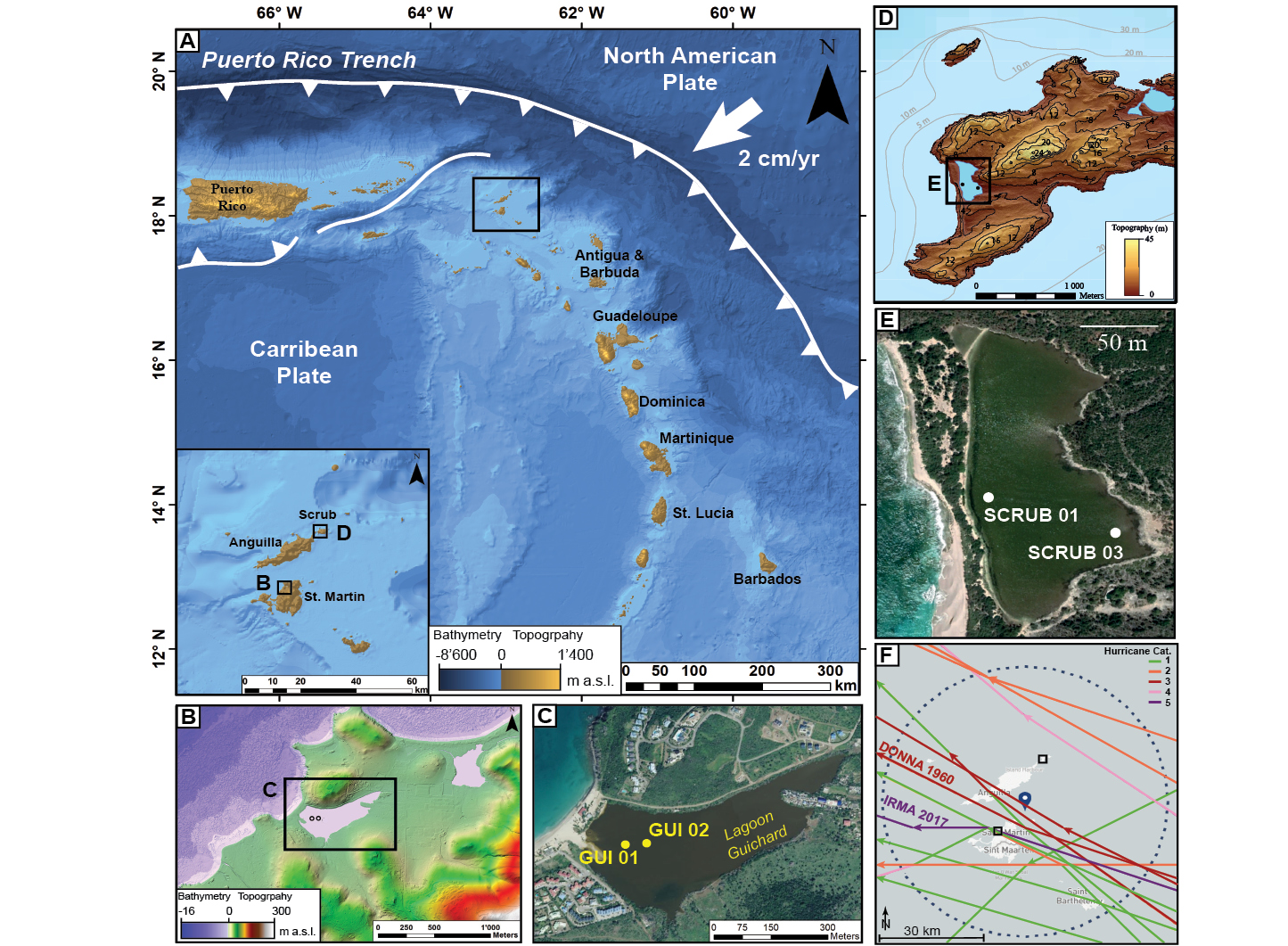
Around 12% of the global population, more than 898 million people in 2020, reside in low-lying coastal areas (≤10 m above sea level; Reimann et al. 2023) that are vulnerable to rising sea level and natural hazards such as hurricanes and tsunamis (MacManus et al. 2021). To prepare for these threats, we must determine the recurrence and intensity of such events beyond instrumental and historical records. Sediment deposits, serving as natural archives, provide vital insights into past tsunamis (e.g. Costa and Andrade 2020) and hurricanes (e.g. Wallace et al. 2021), which are essential for accurate hazard assessment. Coastal lagoon systems are an ideal event archive due to i) their excellent preservation potential as a natural sediment sink, ii) the presence of a sandy barrier separating the ocean from the sink, and acting as a filter for extreme-wave events (EWEs), and iii) their brackish origin, allowing the preservation of inland-mobilized material related to tsunami backwash. Our study investigated sediment cores in coastal lagoons on two Caribbean islands (Saint Martin and Scrub Island) in the Lesser Antilles (Fig. 1).

Earthquake, tsunami and hurricane hazards in the Lesser Antilles

The volcanic arc along the Lesser Antilles was formed by the subduction of the North American Plate under the Caribbean Plate at a rate of 2 cm/yr (Fig. 1a). Although this is one of the most seismically quiet subduction zones worldwide (Cordrie et al. 2022), the area was struck by notable moment magnitudes (Mw) 7 to 8 seismic events, affecting the Caribbean islands over the last 300 years (Feuillet et al. 2011). In addition to intense ground shaking during earthquakes, events in 1843, 1867, 1969, 1985, and 2004 CE generated tsunamis (Cordrie et al. 2022). Historical records and sediment analysis also suggest that the transatlantic Lisbon tsunami of 1755 CE reached the Lesser Antilles, causing tsunami wave heights of more than 2 m, as supported by numerical models (Roger et al. 2011). Apart from earthquakes and tsunamis, the Lesser Antilles islands are also prone to hurricanes, as they are located in the Atlantic hurricane belt. The area of Scrub Island and Saint Martin was struck by 14 hurricanes between 1850 and 2017 CE (NOAA 2020) within a 40 km radius (Fig. 1f). Saint Martin was directly hit by the Category 5 Hurricane "Irma" in September 2017; the strongest hurricane ever formed in the Atlantic zone in historical times (Cangialosi et al. 2018) that broke several meteorological-based records (Fig. 1f). This has spurred research into historical tsunami and hurricane hazards, nurturing efforts to improve our understanding of EWE recurrence intervals and coastal flooding.

Figure 1: (A) Overview of the Lesser Antilles tectonic setting (modified after Biguenet et al. 2021). Inset: Overview of Saint Martin, Scrub Island and neighboring islands showing the investigated coastal lagoons (black squares). The bathymetry and topographic digital elevation model derived from SHOM (2018) for (B) Saint Martin and (C) Scrub Island. Satellite images of the coastal lagoon from (D) Saint Martin and (E) Scrub Island with its sand barriers. (F) Historical hurricane tracks (1850–2017) passing within 40 km (blue dashed circle) of the study area (NOAA 2020).

Methodology for tsunami-and-hurricane deposit analysis

We performed a combination of sedimentological, geochemical, and physical analyses targeting sandy EWE layers for identification and characterization (see Biguenet et al. 2021 and Fabbri et al. 2023 for more details). Furthermore, the cores underwent Loss of Ignition (LOI) and grain-size analyses, which allowed for the identification of variations in grain size, and specific endmembers. Additionally, geochemical analysis using X-ray fluorescence (XRF) was conducted to determine major and trace element contents. X-ray computed microtomography (micro-CT) was used to characterize the sedimentary fabric of EWE deposits (Biguenet et al. 2022; Fabbri et al. 2023). To obtain age constraints on the sediment cores, we developed a chronology based on short-lived radionuclides and radiocarbon ages.

Extreme-wave-event identification and characterization

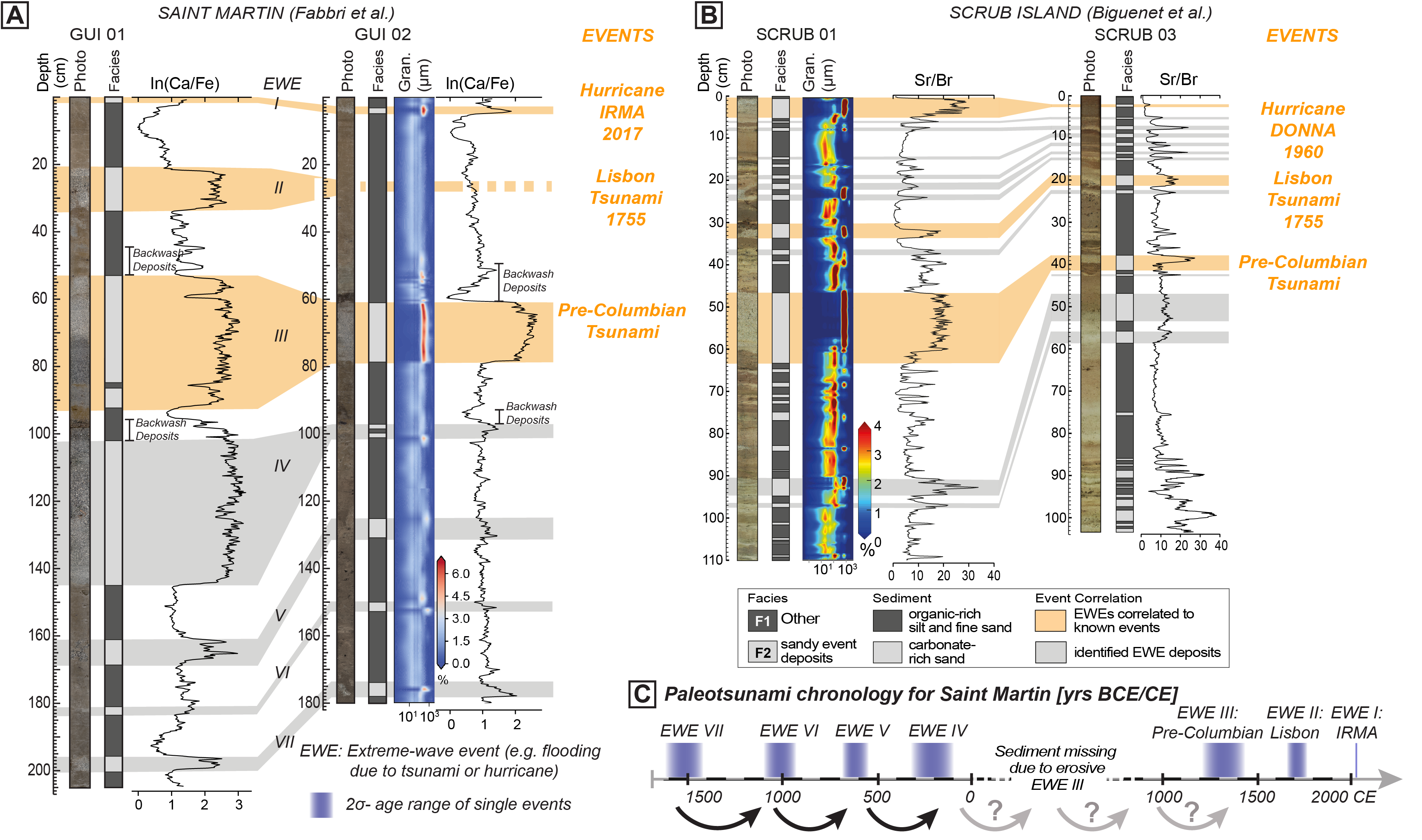
Sedimentological observations and grain-size analysis enabled the identification and distinction of two sediment facies. Facies 1 (F1) is characterized by fine-grained sediment with a silty matrix rich in organic matter (Fig. 2). It contains ~20% organic matter, one-third silicates and a carbonate content between 35% (Scrub Island) and 48% (Saint Martin), reflecting a setting with very low energy levels, and mirroring the lagoon's background sedimentation. In contrast, Facies 2 (F2) comprises significantly coarser sediments, predominantly consisting of fine to very coarse sands. F2 is dominated by carbonates, constituting ~80% at Saint Martin and 40% at Scrub Island, with minor contributions of organic matter. F2's coarse sandy composition, marked by elevated Ca/Fe and Sr/Br ratios, indicates significant marine-sediment input and suggests high-energy transport processes that can erode and resuspend background sediment. Shells and their fragments, rich in Ca or Sr, denote marine influence, while Br and Fe reflects organic matter from the lagoon or land input, respectively. Both ratios represent marine input equally well. Therefore, F2 is interpreted as the facies that likely results from EWEs. Some of the deposits right above the F2 layers (e.g. EWE III) show a geochemical signal rich in fine siliciclastic sediment with organic matter that likely corresponds to backwash deposits (Fig. 2a, b).

Figure 2: Core-to-core correlation of extreme-wave-event (EWE) deposits on (A) Saint Martin and (B) Scrub Island. Photograph, log, sediment facies, grain size and Ca/Fe and Sr/Br ratios shown for event identification. (C) Paleotsunami chronology for Saint Martin with a 400–500 year recurrence interval over the last 3500 years

The EWE deposits characterized by F2 were of primary interest for cross-core correlation. The thickness of F2 layers decreases landward from GUI 01 to 02 at Saint Martin and SCRUB 01 to 03 at Scrub Island, supporting a marine origin of the deposits. Micro-CT-derived sedimentary fabric of event deposits reveals the spatial and geometrical arrangement of their sand grains, offering insights into flow direction and transport medium strength during deposition. A bimodal low-angle fabric dominated the Pre-Columbian tsunami deposit on both islands, distinguishable from the uni- and multi-modal fabric of other EWEs at these sites (Fig. 2). While there is no unique proxy to distinguish between tsunami and hurricane deposits, our recent results show that paleo-flow reconstruction based on micro-CT data may resolve this challenge in the near future.

The recurrence of extreme-wave events

We have identified a total of seven and 25 EWE layers over the last 3500 and 1600 years at Saint Martin and Scrub Island, respectively (Fig. 2). Considering the very small deposit thickness of 1–2 cm of the Category 5 Hurricane Irma at Saint Martin, and the lack of backwash material, older EWEs with thicker deposits must likely be of tsunamigenic origin in this lagoon. This is also supported by CT-derived sedimentary fabric, allowing for a tentative paleotsunami chronology for the island (Fabbri et al. 2023). Moreover, geochemical data (Biguenet et al. 2021) and sedimentary fabric (Biguenet et al. 2022) enabled the identification of two tsunamis among the 25 EWEs on Scrub Island. Scrub Island appears to respond more sensitively to EWEs (including some historic events), compared to the more sheltered Saint Martin lagoon, which is less exposed to the open ocean.

Between 1500 and 0 yr cal BCE, paleotsunamis occurred every 400 to 500 years on Saint Martin (Fig. 2c). The absence of events between 0 and 1350 yr cal CE is likely due to the extensive erosion caused by the Pre-Columbian tsunami, also identified on Scrub Island, and at the regional scale (Cordrie et al. 2022), emphasizing its destructive force. Engel et al. (2016) reported a possible minor event at ~450 yr cal CE, and a major paleotsunami at ~950 yr cal CE, the former observed on Barbados, Yucatan (Mexico), Anguilla and Scrub Island, potentially filling the chronological void. This allows for two potential hypotheses: 1) A regular seismic cycle of strong tsunamigenic earthquakes every 400 to 500 years with a hiatus due to erosion; or 2) Clusters of megathrust earthquakes, referred to as "super seismic cycles", known from many subduction zones and strike-slip faults worldwide (Philibosian and Meltzner 2020), assuming a phase of seismic quiescence instead of a hiatus.

ACKNOWLEDGEMENTS

This work was supported by the Institut France-Québec maritime, the LABEX UnivEarthS project, the Interreg Caraïbes PREST, FEDER (European Community program) and was part of the ANR CARQUAKES project.

affiliationS

1EDYTEM, Université Savoie Mont-Blanc, CNRS, Le Bourget du Lac, France

2Université de Paris, Institut de physique du globe de Paris, CNRS, France

3Institut des sciences de la mer de Rimouski (ISMER), Canada Research Chair in Marine Geology, Université du Québec à Rimouski and GEOTOP, Rimouski, Canada

4Institute of Geological Sciences & OCCR, University of Bern, Switzerland

5LMV, Université Clermont Auvergne, CNRS, IRD, OPGC, Clermont-Ferrand, France

6La Rochelle Université, CNRS, LIENSs, La Rochelle, France

contact

Stefano C. Fabbri: stefano.fabbri@unibe.ch

references

Biguenet M et al. (2021) Sediment Geol 412: 105806

Biguenet M et al. (2022) Mar Geol 450: 106864

Cangialosi JP et al. (2018) Hurricane Irma, NOAA and National Hurricane Center, 111 pp

Cordrie L et al. (2022) Earth-Sci Rev 228: 104018

Costa PJM, Andrade C (2020) Sedimentology 67: 1189-1206

Engel M et al. (2016) Earth-Sci Rev 163: 260-296

Fabbri S et al. (2023) 21st Swiss Geoscience Meeting, Mendrisio, Switzerland

Feuillet N et al. (2011) J Geophys Res Solid Earth 116: B10308

MacManus K et al. (2021) Earth Syst Sci Data 13: 5747-5801

NOAA, (2020) Historical Hurricane Tracks (website), accesed 4 April 2023

Philibosian B, Meltzner AJ (2020) Quat Sci Rev 241(1): 106390

Reimann L et al. (2023) Cambridge Prisms: Coastal Futures 1 (e14): 1-12

Roger J et al. (2011) Pure Appl Geophys 168: 1015–1031

SHOM (2018) MNT bathymétrique de façade de Saint-Martin et Saint-Barthélemy (Projet Homonim)

Wallace EJ et al. (2021) J Geophys Res Letter 48(1): e2020GL091145

We examined multi-proxy evidence preserved within the 2004 Indian Ocean tsunami and overlying 2011 Cyclone Thane deposits on the southeast coast of India. We found no distinguishing features between the deposits.

Over 35% of the Earth’s population lives in coastal zones and is vulnerable to a suite of acute (e.g. storms, cyclones and tsunamis) and chronic (e.g. sea-level rise) coastal hazards (UNEP). Many coastlines and communities are at risk of one or more of these coastal hazards. To properly prepare coastlines that are at risk of these acute coastal hazards, coastal communities and decision makers require detailed knowledge of the occurrence, frequency and magnitude of these events on their coastlines. Fortunately, large storms infrequently impact coastlines, and tsunamis are rare events, but when either event strikes, the outcome can be devastating. Unfortunately, the infrequency of large events makes it challenging for decision makers and communities to prepare.

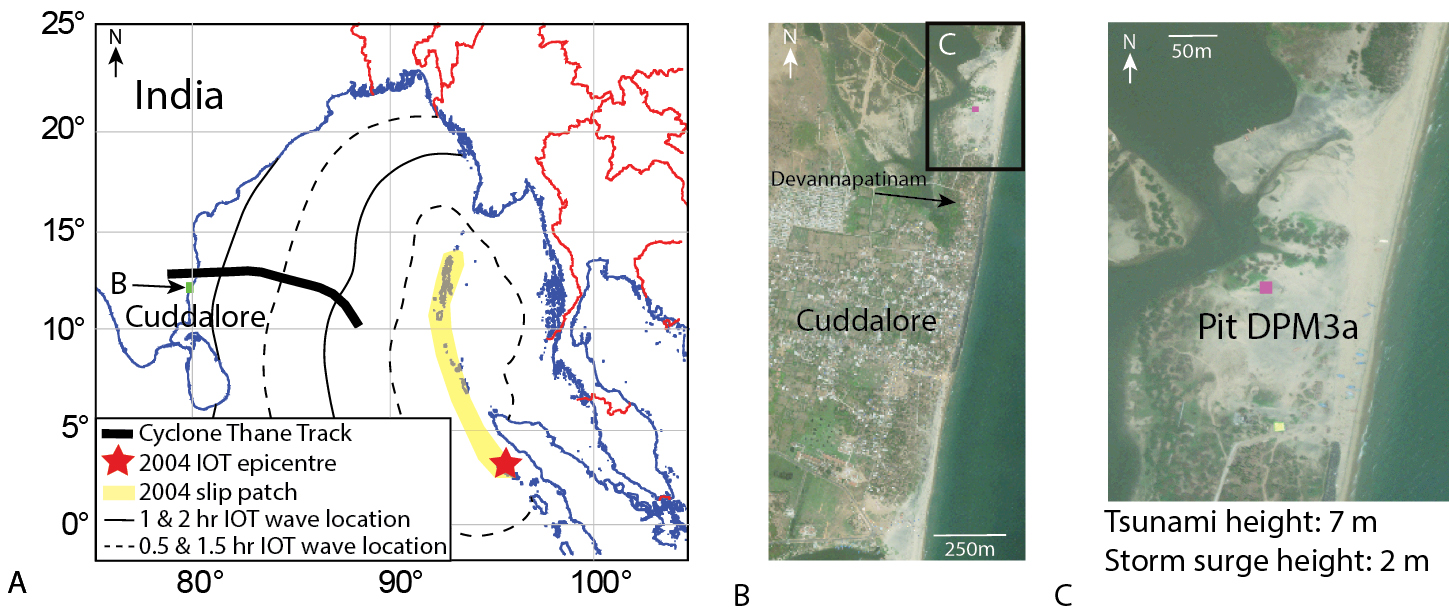
To overcome this challenge, coastal geological records of both depositional and erosional characteristics have been examined to identify signatures of past coastal hazards (e.g. Switzer et al. 2014). These studies typically focus on areas where a coastal hazard has been encountered (e.g. Jankaew et al. 2008). However, to appropriately identify which coastal hazard has affected a region, modern analogues must be examined to identify characteristics that are unique to each hazard (e.g. Morton et al. 2007). Although much effort has focused on distinguishing between storm and tsunami characteristics in the geological record, these studies have examined deposits of tsunami and storms from different coastlines (e.g. Kortekaas and Dawson 2007; Morton et al. 2007), or have examined deposits that have occurred decades apart and may have undergone alteration (e.g. Nanayama et al. 2000). To date, very few studies have examined the geological signatures of a known tsunami and known storm deposit from the same location (e.g. Pham et al. 2017; Yap et al. 2021). We contribute to this growing body of knowledge by examining the beautifully preserved sedimentary deposits formed by the 26 December 2004 Indian Ocean tsunami (IOT), and the 2011 Cyclone Thane from Devanampattinam on the northern outskirts of Cuddalore, southeast India (Fig. 1a).

The 2004 tsunami and the 2011 cyclone

The 2004 IOT was triggered by a magnitude moment 9.2 earthquake centered off northeastern Sumatra and propagated northwards along 1500 km of the Sumatran–Andaman subduction zone, killing 230,000 people (Fig. 1). The IOT propagated across the Bay of Bengal and struck southeast India at 8:30 a.m. local time, causing approximately 16,000 deaths and US$2 billion (International Recovery Platform 2004). At Devannampatinam, the tsunami had a maximum run-up height of 7 m and 700 m of inundation; and deposited a 38 cm thick sediment deposit.

Cyclone Thane made landfall near Cuddalore between 6:30 and 7:30 a.m. on 30 December 2011, causing over US$1 billion in damage and killing 48 people (Fig. 1; IMD 2012). At Devannampatinam, the storm surge run up was approximately 2 m, inundated approximately 300 m and deposited 27 cm of sediment.

Comparison of Cyclone Thane and 2004 IOT sedimentary deposits

Figure 1: (A) Map of the Bay of Bengal showing the location and travel times of the 2004 IOT and Cyclone Thane storm track. (B) Satellite image of the Cuddalore coast showing the location of Devannampatinam and the pit site. (C) Satellite image of the beach near Devanampattinam where pit DPM3a was excavated.

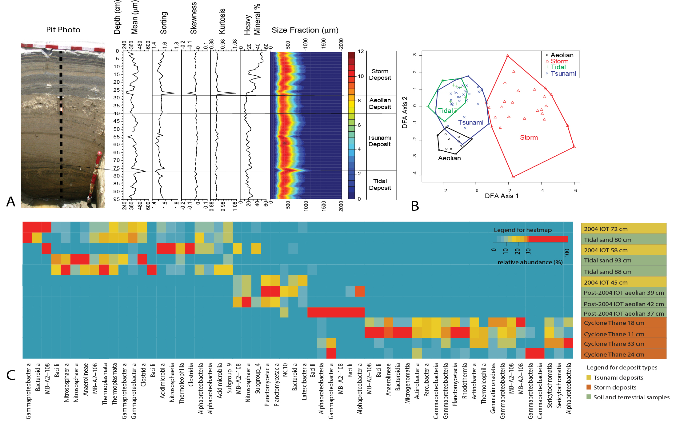
Using satellite imagery of the region and discussions with local survivors, we identified a site approximately 300 m north of the village of Devannampatinam that preserves the 2004 IOT and 2011 Cyclone Thane deposits (Fig. 1a). The site was a partially vegetated; sandy beach dunes and backshore lagoonal environments formed from the closure of the Pennai River. At this site we excavated the 95 cm deep pit DPM3a and conducted multi-proxy analysis at centimetre-scale resolution that included stratigraphy, sediment grainsize, grain shape, and heavy mineral counts (Fig. 2a). Multivariate statistical analysis of the sedimentary variables demonstrates distinct differences between storm and tsunami deposits (Fig. 2b). We analyzed the microbial communities of 26 samples from the pit (Yap et al. 2021), but present the results of 13 representative samples here (Fig. 2c).

From deepest to shallowest, the sedimentary units observed in Pit DPM3a are an intertidal sand, 38 cm thick 2004 IOT deposit, a 12 cm thick layer of eolian (wind blown) sand, and the 27 cm thick Cyclone Thane deposit (Fig. 2a). All of the units consist of medium sands (average size from 0.25–0.5 mm). The intertidal unit consists of northward dipping beds and thin horizontal beds, both with distinct heavy mineral layers (10–30%; Fig. 2a). The tsunami deposit consists of two beds separated by thin heavy-mineral laminations. From the bottom to the middle of the beds, the grain size becomes larger, and from the middle of the beds the grain size becomes smaller (Fig. 2a). These two beds represent deposition from two sequential waves, and much of the sediment came from the pre-existing nearshore or onshore environments. The eolian deposit consists of sands that have been partially reworked upper-2004-IOT sediments, some leaves and plastic waste (Fig. 2a). The storm deposit is composed of horizontal layers that consist of different proportions of heavy minerals (15–60%). The layers are thicker at the bottom of the deposit and become thinner towards the top. It is likely that the sediments came from the shoreface or onshore environments (Fig. 2a).

Discriminant function analysis (DFA) of all four deposits indicates that sedimentologically, only the heavy mineral distribution in the storm deposit can distinguish the four units (Fig. 2b). However, at Silver Beach, less than 2 km south of Devanampattinam, Srinivasalu et al. (2007) and Switzer et al. (2012) described 2004 IOT deposits with abundant heavy minerals and dense laminations, in contrast with Pit DPM3a.

Figure 2: (A) Sedimentological parameters of Pit DPM3a. (B) DFA of sediment grain-size characteristics and heavy-mineral content of DPM3a units. (C) Microbes heatmap showing the relative abundances of different microbial groups in DPM3a communities. Figure modified from Yap et al. 2021.

Comparison of Cyclone Thane and 2004 IOT microbial communities

Analysis of microbial communities followed standard procedures of extracting deoxyribonucleic acid (DNA) sequences from the sediment (Yap et al. 2021). Microbial metabarcoding analysis performed in this study targets the 16S ribosomal ribonucleic acid (rRNA) gene that identifies archaea, bacteria and eukaryotic taxa, as well as the 18S rRNA gene that is primarily used for identifying eukaryotic taxa. These rRNA markers are functionally similar over evolutionary time within a species, but exhibit variation across different species. The amplified DNA (called an amplicon) is then sequenced through a next-generation sequencer that generates a vast amount of DNA-sequence data. The distinct structure of the DNA sequences are determined (called amplicon sequencing variants – ASVs), and these ASVs are taxonomically distinct, thereby representing different species. Grouping of the average 42,406 DNA sequences resulted in a total of 4971 unique ASVs.

The microbial communities in the Cyclone Thane deposit significantly differed from the microbial communities in the 2004 IOT deposit, whereas the microbial communities within the 2004 IOT deposit were not significantly different from the underlying intertidal and overlying eolian deposits (Yap et al. 2021). The unique taxa preserved in the Cyclone Thane deposit included taxa from the families Chromobacteriaceae, Rubinisphaeraceae, Burkholderiaceae, Micromonosporaceae, Bacillaceae, Nocardioidaceae, Sporichthyaceae, Caulobacteraceae, and Chitinophagaceae, classes Sericytochromatia and Thermoplasmata, and the phylum Parcubacteria (Fig. 2b). No eukaryotic taxa could distinguish between the Cyclone Thane and 2004 IOT deposits.

Although it seems promising that storm and tsunami deposits can be distinguished by their microbial communities, further examination of another modern storm deposits on Phra Thong Island, Thailand, revealed that only taxa from the family Chitinophagaceae and class Thermoplasmata were present in both deposits (Yap et al. 2021). Further analysis of modern storm deposits may confirm the global signature of these taxa as unique to storm deposits. As no unique tsunami microbial signatures were present in the 2004 IOT deposits in India or Thailand, it is apparent that no global microbial signature exists for tsunami deposits (Yap et al. 2021).

This analysis focused on developing modern microbial signature analogues from storm and tsunami deposits. However, the microbial communities identified from the stacked 2004 and paleotsunami deposits from Thailand clearly show that the microbial communities become homogenized with non-tsunami sediments with age (Yap et al. 2023). It is likely the same would occur with older storm deposits under similar environmental conditions.

From our analysis of the 2011 Cyclone Thane and 2004 IOT deposits on the southeast coast of India, the sedimentological, stratigraphic and environmental DNA can discriminate recent coastal overwash events. However, modern analogues of both storm and tsunami deposits from the same geographical area are required to accurately discriminate between storm and tsunami deposits preserved in the geological record.

affiliationS

1Research School of Earth Sciences, Australian National University, Canberra, Australia

2Earth Observatory of Singapore, Nanyang Technological University, Singapore

3Asian School of the Environment, Nanyang Technological University, Singapore

4Insitute of Ocean Management, Anna University, Chennai, India

5National Institute of Ocean Technology, Chennai, India

6VNU University of Science, Vietnam National University, Ha Noi, Vietnam

*These two authors contributed equally to this work

contact

Chris Gouramanis: chris.gouramanis@anu.edu.au

references

IMD (2012) Very Severe Cyclonic Storm "THANE" over the Bay of Bengal (25-31 December, 2011): A Report. Cyclone Warning Division, Ministry of Earth Sciences, Government of India, New Delhi, 10 pp

International Recovery Platform (website), accessed 6 April 2011

Jankaew K et al. (2008) Nat 455: 1228-1231

Kortekaas S, Dawson AG (2007) Sed Geol 200: 208-221

Morton RA et al. (2007) Sed Geol 200: 184-207

Nanayama F et al. (2000) Sed Geol 135: 255-264

Pham DT et al. (2017) Mar Geol 385: 274-292

Srinivasalu S et al. (2007) Mar Geol 240: 65-75

Switzer AD et al. (2012) Geol Soc Lond, Spec Pub 361: 61-77

Switzer AD et al. (2014) J Coastal Res 70: 723-729

UNEP (website), Coastal Zone Management, accessed 23 October 2023

Yap W et al. (2021) Comms Earth & Environ 2: 129

Yap W et al. (2023) Mar Geol 457: 106989

X-ray fluorescence (XRF) analysis is a geochemical technique that reveals subtle environmental changes over sub-annual to millennial timescales. Elemental geochemistry of salt-marsh sediments responds to tidal frequency similar to microfossil distributions, which are used to reconstruct sea- and land-level change.

Subduction zones are known to generate some of the largest magnitude earthquakes and their subsequent tsunamis are capable of inundating local and distant coastlines. The recurrence interval of large earthquakes rupturing along a subduction interface are generally on the order of hundreds to thousands of years, making risk assessment challenging because the observational records do not fully capture these larger timescales (e.g. Sawai et al. 2012). Therefore, we must rely on the geologic record to extend our understanding of earthquake-rupture mechanisms, magnitudes, and frequencies (e.g. Atwater et al. 2003; Nelson et al. 2021).

Salt-marsh archives

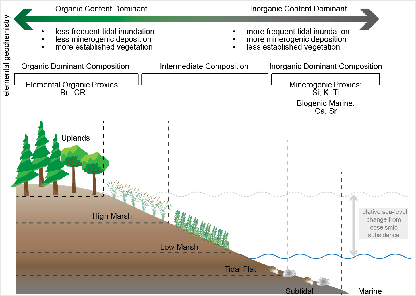
In salt marshes, tides result in distinct environmental zones that are controlled by the frequency and duration of tidal inundation. Tidal inundation in salt marshes is controlled by the elevation gradient relative to sea level; where lower elevations are inundated more frequently and for longer durations than sections of the marsh situated at higher elevations. The predictable response of salt-marsh sediments to tidal inundation forms the basis for applying proxies (i.e. microfossils, XRF-elemental geochemistry) to reconstruct sea-level change, and in doing so, identifying paleoearthquakes and tsunamis in the geologic record (Atwater and Hemphill-Haley 1997).

In salt marshes, megathrust earthquakes may result in coseismic subsidence (instantaneous land-level lowering during the earthquake), which is analogous to instantaneous local sea-level rise. Stratigraphically, coseismic subsidence is identified as peat-mud couplets where pre-earthquake intertidal peat is suddenly lowered further into the intertidal and subtidal zone, where mud is subsequently deposited, resulting in a distinctive mud-over-peat contact (Atwater 1987). The tsunami generated from the earthquake can also inundate local coastlines, and the resulting overwash sediments can be preserved within salt-marsh stratigraphy as a thin marine sand sheet between the peat (pre-earthquake) and mud (post-earthquake) units (Hemphill-Haley 1995).

XRF as a tool for recognizing paleoearthquakes and tsunamis

Although intertidal microfossils (e.g. foraminifera and diatoms) are among the most widely used proxies for reconstructing paleoearthquakes and tsunamis (Pilarczyk et al. 2014), elemental geochemistry obtained through XRF-core scanning (XRF-CS) is a promising technique for reconstructing long term records of coastal change because of its rapidness and ability to detect even subtle environmental changes preserved within sediment cores (Giang et al. 2023).

XRF-CS offers rapid, continuous and non-destructive analysis of elemental composition for a wide range of geologic materials, including core samples. In XRF analysis, samples are irradiated with X-rays which induce the atoms from the samples to emit characteristic fluorescence photons. Detectors measure the energies of fluorescence photons which, in turn, identify the element and the number of fluorescence photons of that energy, to determine the abundance of a particular element in a given substance.

In theory, XRF analysis identifies all elements based on their characteristic fluorescence emissions, but in practice, XRF is incapable of detecting low atomic number elements (Z <11; e.g. H, C, N, O). Instead, XRF can indirectly measure these elements based on the X-ray scatter measured simultaneously with elemental data. X-ray scatter occurs when an incident X-ray is redirected or changes direction due to an interaction with an electron. Incoherent scattering occurs when the X-ray loses energy to the electron and is more prevalent with lower atomic number elements, while coherent scattering involves no change in X-ray energy and is more common with higher atomic number elements. The incoherent/coherent scattering ratio (ICR) provides insights into the average atomic mass of the total elemental composition.

Along salt-marsh coastlines, the elemental composition of modern marsh sediments shows a consistent relationship with tidal elevation, and is in agreement with marsh zones that are derived from intertidal microfossil assemblages (Giang et al. 2023; Pilarczyk et al. 2014). Generally, tidal flat and low marsh sediments from lower elevations are dominated by lithogenic (Si, K, Fe, Ti) and biogenic (Ca, Sr) elements (Fig. 1). At low elevations, frequent tidal inundation remobilizes detrital sediment from the subtidal basin into the intertidal salt marsh. At higher elevations, the elemental composition is dominated by Br (high marsh; Fig. 1); however, despite its high abundance in seawater, Br in marshes is not as dominant at low elevations, but rather at high elevations where tidal inundation is less. This may be the result of Br’s involvement in biogeochemical processes that transform mobile Br ions into immobile species within peats and soils (e.g. Keppler et al. 2000).

Figure 1: Conceptual model of elemental geochemistry zonation within Cascadia salt marshes. The elemental composition of low elevation (i.e. tidal flat) sediments is dominated by lithogenic (Si, K, Ti, Fe) and biogenic (Ca, Sr) elements, while the composition at high elevations (i.e. high marsh/uplands) is dominated by organic indicators, such as Br and ICR (incoherent/coherent scattering ratio). Relative sea-level change associated with coseismic subsidence is shown in gray, and results in the deposition of tidal flat muds on top of salt-marsh peats.

The ICR is applied as a proxy for organic content because organic forming elements (e.g. H, C, O, N) tend to have lower atomic numbers, while clastic sediments tend to be composed of higher atomic number elements (e.g. Si, Fe) (Woodward and Gadd 2019). The ICR also follows the same trend as Br, where highest values are found at high elevations where vegetation is most established within the intertidal range (Fig. 1). The elemental composition can distinguish subtle differences in the inorganic and organic content of salt-marsh sediments, which is predominantly controlled by tidal inundation.

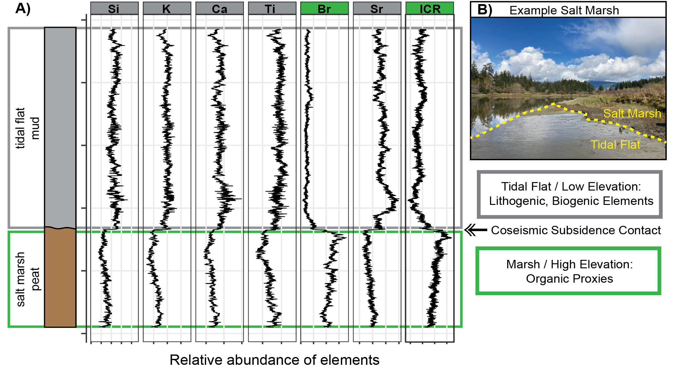
Elemental geochemistry, obtained through XRF analysis, can resolve continuous, high-resolution elemental variation within sediment cores (Fig. 2). The relationship between modern salt-marsh sediments and elemental geochemistry can be applied downcore to resolve changes in paleoenvironmental conditions, including sudden, high-magnitude changes, such as coseismic subsidence associated with large earthquakes as shown conceptually in figure 2. Coseismic subsidence may be recognized by a dramatic and sharp change in geochemistry from an organic dominated composition (i.e. Br-rich peats, soils) to a lithogenic and biogenic dominated one (i.e. Si, K, Fe, Ti, Ca, and Sr-rich tidal flat mud; Fig. 2). Elemental geochemistry may be especially useful for recognizing smaller amounts of coseismic subsidence when stratigraphic evidence is not obvious. Data derived from XRF analysis may also be applied as a supplemental proxy in microfossil-based sea- and land-level reconstructions to increase precision (e.g. Cahill et al. 2016). The downcore applications of elemental geochemistry for reconstructing coseismic subsidence still requires ground truthing, but shows promising potential based on the modern relationship between elemental composition and tidal elevation of salt-marsh sediments (Giang et al. 2023).

In addition to delineating the occurrence of coseismic subsidence in marsh stratigraphy, elemental geochemistry can also be used to identify tsunamis. Tsunami sediments preserved in salt marshes are often characterized by high concentrations of seawater ions (e.g. Na+, Cl-) and heavy elements from the offshore environment (e.g. Zn, Pb) (Chagué-Goff et al. 2017). In this way, XRF data can identify a marine origin for the anomolous sands, and may provide better estimates of marine inundation limits and lateral extensiveness of these deposits.

Figure 2:  (A) Idealized sediment core collected from a salt marsh and associated conceptual elemental data illustrating stratigraphic evidence for coseismic subsidence. The subsidence contact is recognized by a sharp and abrupt change in lithology and elemental composition. Lithogenic (Si, K, Ti,) and biogenic (Ca, Sr) elements dominant at low elevations are highlighted in gray, while organic elements (Br, ICR), dominant at high elevations, are highlighted in green. (B) Typical Cascadia salt marsh where evidence for earthquakes and tsunamis can be found. The tidal flat and salt marsh subenvironments are delineated with the dashed line.

Advantages of elemental geochemistry

XRF-CS analysis simultaneously measures a wide suite of elements (Al to U), each with the potential to bolster paleoenvironmental and sea-level reconstructions. The rapid and high resolution (up to 100 µm) capability of the XRF-CS, in particular, enhances our ability to detect subtle changes occurring over very short timescales. Similarly, XRF-CS offers non-destructive analysis of sediment cores, allowing for flexibility in subsampling strategies where elemental geochemistry can help guide subsequent destructive analyses (e.g. microfossil and grain-size analysis). Elemental geochemistry has many unexplored, but promising, applications that can be applied to the study of paleoearthquakes and tsunamis.

ACKNOWLEDGEMENTS

This article is a contribution to IGCP Project 725 "Forecasting Coastal Change" and INQUA CMP.

affiliationS

1Department of Earth Sciences, Simon Fraser University, Burnaby, Canada

2Department of Geography and the Environment, Villanova University, USA

contact

Anthony Giang: anthony_giang@sfu.ca

references

Atwater BF et al. (2003) In: Developments in Quaternary Sciences. Elsevier, 331-350

Atwater BF (1987) Science 236 (4804): 942-944

Atwater BF, Hemphill-Haley E (1997) US Geol Surv Prof Pap 1576, 108 pp

Cahill N et al. (2016) Clim Past 12: 525-542

Chagué-Goff C et al. (2017) Earth-Sci Rev 165: 203-244

Giang A et al. (2023) MSc Thesis, Simon Fraser University, 63 pp

Hemphill-Haley E (1995) Geol Soc Am Bull 107: 367-378

Keppler F et al. (2000) Nature 403: 298-301

Nelson AR et al. (2021) Quat Sci Rev 261: 106922

Pilarczyk JE et al. (2014) Palaeogeogr Palaeoclimatol Palaeoecol 413: 144-157

Sawai Y et al. (2012) Geophys Res Lett 39: L21309

Woodward CA, Gadd PS (2019) Quat Int 514: 30-43

Diatoms form a powerful proxy for reconstructing subduction-zone earthquake and tsunami histories. Using examples from Chile, we explore what diatoms have been able to tell us to ultimately help improve seismic hazard assessment, and highlight challenges and opportunities.

Globally, great subduction-zone earthquakes (moment magnitude [Mw] >8), and the tsunamis they generate, produce cascading hazards along coastlines. As the largest events can be so devastating, yet so infrequent, geologic records of earthquakes and tsunamis spanning centuries to millennia are required to understand subduction-zone behavior, and account for variability in earthquake size, rupture style and tsunami generation. Coastal sediments are excellent recorders of past earthquakes and tsunamis, and microfossils, such as diatoms (siliceous single-celled algae) found within them, have become one of the most commonly used proxies for reconstructing subduction-zone earthquake and tsunami histories (Dura et al. 2016).

Since the seminal work in the Pacific Northwest (e.g. Atwater 1987; Darienzo and Peterson 1990), the last 40 years have seen major advances in diatom-based reconstructions of earthquakes and tsunamis (Dura et al. 2016). Due to the close control of salinity on diatom distribution in intertidal environments, diatoms can be used to quantify vertical land-level change associated with great earthquakes, not only coseismically during earthquakes, but also potential pre- and post-earthquake deformation. Due to their resistance to degradation, diatoms have also been widely used to determine the provenance of tsunami sediments and changing flow conditions during tsunamis. Here we review three case studies from the Chilean coast that demonstrate how diatoms are being used to reconstruct earthquake and tsunami history on a highly active subduction zone, and highlight important lessons from our research.

Extending historical records

At Chucalén, south-central Chile, in the centre of the area which ruptured in the world’s largest instrumentally recorded earthquake, a Mw 9.5 event in 1960 CE, diatoms formed a powerful proxy for reconstructing coseismic land-level change that occurred in that event, and three earlier earthquakes during the last millennium (Fig. 1; Garrett et al. 2015). Diatom-based estimates of coseismic land-level change varied for the four earthquakes, ranging from meter-scale subsidence to slight uplift, suggesting variability in slip distribution. The length of the paleoseismic record at Chucalén is twice as long as the historical record, yet historically documented events in 1737 and 1837 CE are absent, critically suggesting variability in magnitudes and longer recurrence intervals between the largest events.

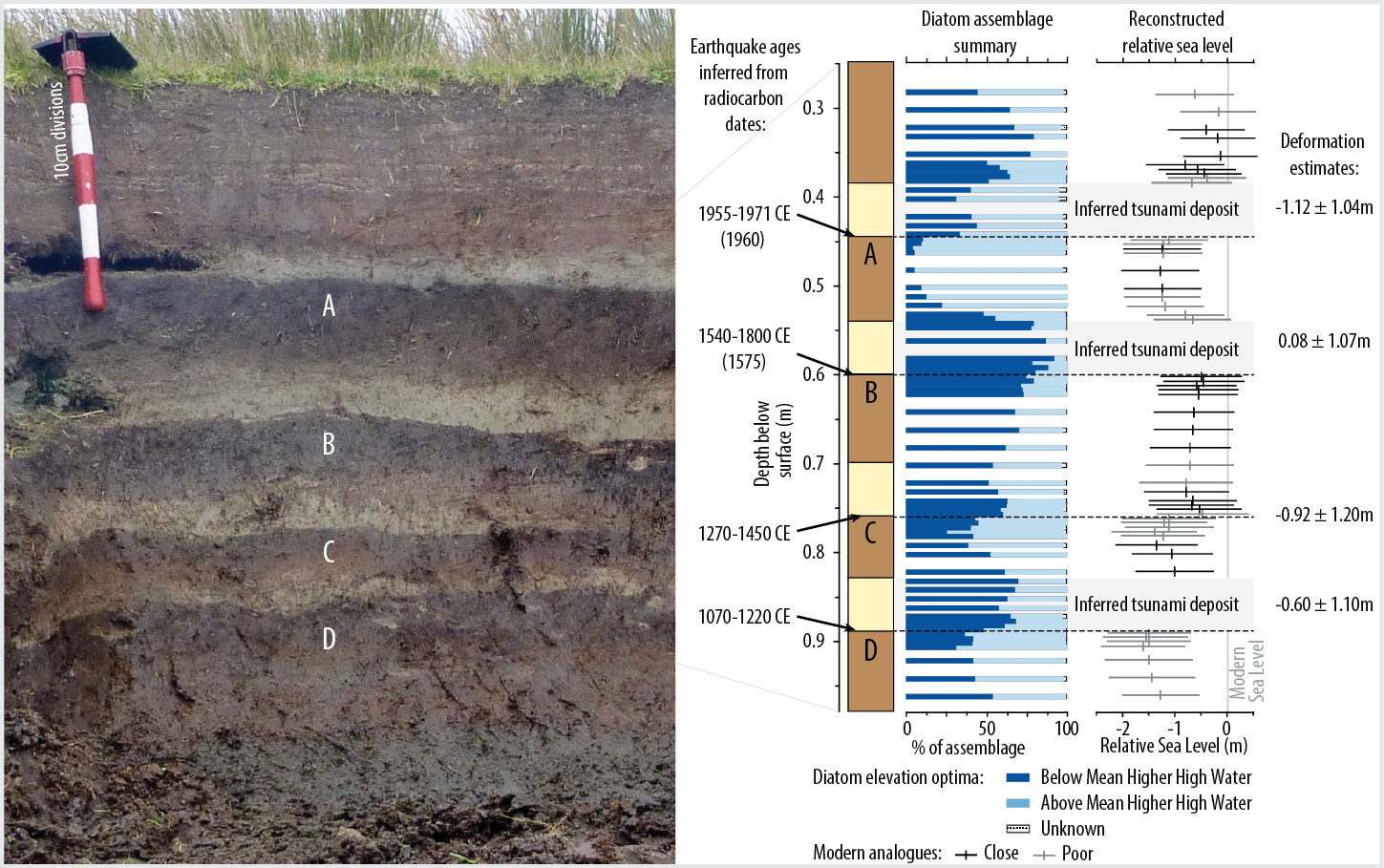Figure 1: A 1000-year record of great earthquakes at Chucalén, south-central Chile, shown by the laterally extensive buried soils (A–D) and diatoms. Figure modified from Garrett et al. (2015).

The importance of utilizing multi-proxy geological and historical evidence in tandem

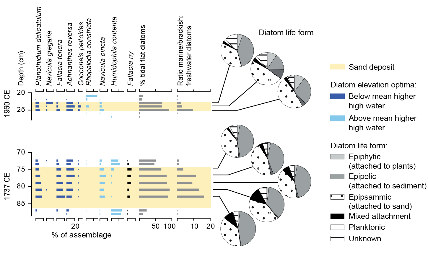
Historical records most commonly used in assessing seismic hazards are often too short to account for variability in earthquake size, rupture style and tsunami generation. Moreover, even where long written chronicles exist, failures in reporting, loss of documents in times of political instability or low-quality records may result in temporal gaps. Albeit with other limitations, geologic records are free from these problems. An example from Chaihuín, south-central Chile, close to the region of maximum slip in 1960 CE, demonstrates that it is imperative to supplement historical data with geologic records (Hocking et al. 2021).

Previously, the lack of reports of tsunami inundation from the 1737 CE south-central Chile earthquake had been attributed to either civil unrest (which restricted Spanish settlers from occupying all, bar two, coastal towns) or a small tsunami due to deep-fault slip below land. However, using sedimentological and diatom analyses of tidal marsh sediments, we found evidence for a previously unreported, locally sourced tsunami consistent in age with this event. Diatoms confirmed coseismic subsidence of up to 0.9 m and abrupt marine inundation (Fig. 2). Coupled dislocation-tsunami models placed the causative fault slip mostly offshore, rather than below land, and our findings reduced the average recurrence interval of tsunami inundation derived from historical records alone.

Figure 2: Sand deposits at Chaihuín, south-central Chile, dominated by marine and brackish diatoms characteristic of low elevations, provide evidence for marine-sourced sand and rule out fluvial deposition. In combination with sedimentological evidence and coincident subsidence discounting storm-surge origin, sand layers are interpreted as tsunami deposits.

The importance of millennial-scale geologic records in characterizing earthquake and tsunami hazards

In central Chile, historical accounts, and later instrumental measurements of a series of ~Mw 8.0–8.5 earthquakes and low (<4 m) tsunamis affecting the region in 1575, 1580, 1647, 1730, 1822, 1906 and 1985 CE, suggest a consistent recurrence interval of ~80 years for large earthquakes in the region. However, more recently uncovered historical clues from the 1730 CE event suggest this earthquake was larger (>Mw 9) than other earthquakes in the historical series, and produced a high tsunami that affected both the Chilean and Japanese coasts (Carvajal et al. 2017).

To dig deeper into the history of past >Mw 9 earthquakes along the densely populated central Chilean coast, Dura et al. (2015) conducted a stratigraphic, sedimentological and diatom investigation at Quintero. The study found evidence of six instances of high tsunami inundation and coastal uplift between 6200 and 3600 cal yrs BP, similar to that documented in 1730 CE. Diatom data were critical to supporting a marine source of the anomalous sand beds found in the stratigraphy, and for estimating uplift of ~0.5 m in each earthquake. The new tsunami and land-level change evidence shows a recurrence interval of ~500 years for outsized earthquakes and tsunamis in central Chile, and demonstrates that basing hazard assessments on only the most recent, but smaller, earthquakes and tsunamis overlooks the higher hazard posed by less frequent, but larger, events.

Challenges, opportunities and outlook

The examples demonstrate the value of utilizing diatoms in paleoseismology. However, as with any proxy, there remain challenges associated with their application. First, the above examples adopt transfer functions to quantify land-level change and, whilst such approaches enable more precise estimations of land-level change than earlier qualitative assessments, transfer functions have inherent assumptions and limitations. Diatom taxa in fossil sediments that are not present in our modern datasets (non-analogue situations) limit our ability to reconstruct past environmental change and accurately quantify land-level change.

Modern diatom dataset development is particularly challenging in places that have recently undergone coseismic subsidence, as the present-day tidal marsh may not provide a good modern analogue for the entire fossil sequence. Every effort must be made to improve modern diatom datasets by increasing numbers of samples across a range of coastal environments (capturing the full gradients of elevation, vegetation, substrates) to help mitigate against non-analogue situations (Hocking et al. 2017). Even then, reconstructions can be complicated by reworked microfossils, with certain taxa being prone to transport across the intertidal zone, and thus not being representative of their depositional environment (Hemphill-Haley 1995). In such instances, it may be necessary to exclude specific taxa when performing reconstructions. We emphasize that improved understanding of relationships between diatoms, salinity and substrates in the modern environment, as well as variations in the preservation and transport of specific taxa, will ensure more reliable identification of earthquakes and tsunamis in the geological record, and quantification of land-level change.

There is also the assumption when quantifying land-level change using a transfer function that sedimentary hiatuses do not occur post-earthquake. If sediment accumulation does not recommence before significant postseismic deformation occurs, the magnitude of coseismic deformation may be underestimated in transfer function reconstructions. Such delay in postseismic sediment accumulation was observed at two sites following the 2010 CE earthquake (Garrett et al. 2013), and the duration of such hiatuses are difficult to identify in fossil records.

Finally, as well as potentially underestimating the magnitude of deformation, geologic records may also underestimate the occurrence of Mw 7–8 earthquakes. Diatom analyses of tidal-marsh sediments within the rupture area of the 2016 CE Mw 7.6 Chiloé earthquake, south-central Chile, showed records of low-level (<0.1 m) land-level change were created for a limited period of time in limited parts of the tidal wetland, following the earthquake, with statistically significant changes observed between diatom assemblages pre- and immediately post-earthquake (Brader et al. 2021). However, the signal was temporary, and after nine months such assemblage changes were not preserved due to sedimentation processes (Brader et al. 2021). This highlights the limits of detection of this microfossil-based technique, and the potential underestimation of major, but not great, earthquakes in coastal paleoseismological records. This has important implications for estimating recurrence intervals in seismic hazard assessment, and further highlights the need to utilize multiple lines of evidence.

Diatoms are extremely useful for quantifying land-level change associated with subduction-zone earthquakes, and for determining tsunami provenance, ultimately helping to better understand recurrence intervals and variability in ruptures. However, their application must be seen as a key component of the paleoseismology toolkit; other proxies, as well as other approaches to reconstructing past earthquakes and tsunamis, such as the use of documentary evidence and modeling, are equally important. The power comes from combining approaches, and through such multidisciplinary research we can continue the remarkable advances in seismic-hazard assessment which have occurred over the last decade.

ACKNOWLEDGEMENTS

We acknowledge the contribution of co-authors to research presented here, including M. Cisternas, D. Melnick, D. Aedo, M. Carvajal, L. Ely, R. Wesson, I. Shennan, M. Brader, and funding from NERC, EU, and NSF.

affiliations

1Department of Geography and Environmental Sciences, Northumbria University, Newcastle-upon-Tyne, UK

2Department of Environment and Geography, University of York, UK

3Department of Geosciences, Virginia Tech, Blacksburg, USA

contact

Emma P. Hocking: emma.hocking@northumbria.ac.uk

references

Atwater BF (1987) Science 236 (4804): 942-944

Brader M et al. (2021) J Quat Sci 36: 991-1002

Carvajal M et al. (2017) J Geophys Res: Sol Earth 122: 3648-3660

Darienzo ME, Peterson CD (1990) Tectonics 9: 1-22

Dura T et al. (2015) Quat Sci Rev 113: 93-111

Dura T et al. (2016) Earth-Sci Rev 152: 181-197

Garrett E et al. (2013) Quat Sci Rev 75: 11-21

Garrett E et al. (2015) Quat Sci Rev 113: 112-122

Hemphill-Haley E (1995) Geol Soc Am Bull 107: 367-378

Hocking EP et al. (2017) J Quat Sci 32: 396-415

Hocking EP et al. (2021) Commun Earth Environ 2: 245

Diatoms are invaluable to subduction-zone paleoseismic studies due to their ability to provide a continuous record of coseismic, postseismic and interseismic deformation, helping to better define the spatial variability of seismicity over centennial to millennial timescales.

Recent GPS instrumentation and Interferometric Synthetic Aperture Radar (InSAR) observations, coupled with increasingly sophisticated modeling, have identified complex patterns of subduction-zone deformation during earthquakes (coseismic), immediately after earthquakes (postseismic), and in between earthquakes (interseismic) (e.g. Klein et al. 2017). However, GPS and InSAR datasets span only decades, which is a fraction of the hundreds to thousands of years great earthquake cycle. Thus, the degree to which they reflect long-term rates of deformation is widely debated (Sieh et al. 2008). Are modern measurements and observations of subduction-zone earthquakes and tsunamis consistent with past events and, thus, reliable indicators of the future behavior of the subduction zone? Coastal paleoseismic studies that reconstruct rupture histories over multiple earthquake cycles suggest that the answer to this question is no, and that relying on short instrumental and historical earthquake and tsunami observations can lead to devastating societal impacts (Philibosian and Meltzner 2020; Witter et al. 2016).

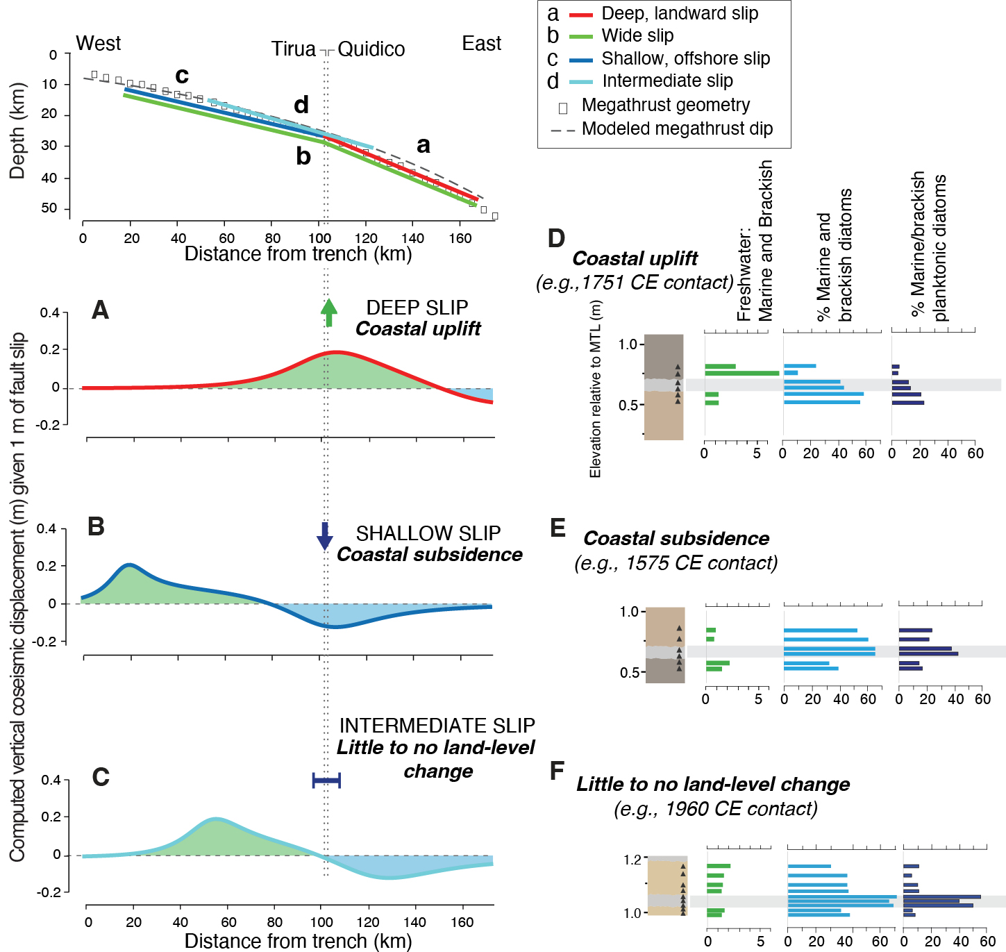Figure 1: A simple model of constant coseismic slip and corresponding vertical deformation on a subduction zone in which slip is confined to a (A) deep; (B) shallow; or (C) intermediate zone. (D) An example of the diatom response to coastal uplift; (E) coastal subsidence; and (F) little to no coastal deformation. Figure and caption are modified from Dura et al. (2017).

Coastal paleoseismic studies, which use the methods of coastal stratigraphy, sedimentology, micropaleontology, and geophysical and sediment transport modeling to reconstruct vertical tectonic deformation along subduction zones coasts, have proven to be a powerful tool for examining the earthquake deformation cycle over centennial to millennial timescales. Past earthquakes are expressed in tidal wetland stratigraphy as sharp stratigraphic contacts between organic-rich peat below the contact, and tidal mud above (coseismic subsidence), or between tidal mud below the contact and organic-rich peat above (coseismic uplift) (Atwater 1987; Dura et al. 2017). The stratigraphic transitions captured in between earthquakes reflect the postseismic and interseismic period of the earthquake deformation cycle. Microfossils, such as diatoms, preserved in tidal wetland stratigraphy can provide quantitative estimates of the vertical surface deformation associated with the subduction-zone earthquake cycle (Shennan and Hamilton 2006). Diatom assemblages (groups of diatom species) are particularly useful in paleoseismic studies because their sensitivity to differences in tidal inundation, substrate and salinity can be precisely related to elevation within the tidal frame (Dura et al. 2016). Quantitative models, termed transfer functions, can be constructed from the relative abundance of diatom assemblages at modern tidal-marsh elevations, which can then be applied to diatom assemblages found in cores and/or outcrops, to reconstruct the elevation of a sample when it was deposited. Transfer function analysis can provide a continuous record of coseismic, postseismic and interseismic deformation along subductions zones (e.g. Hawkes et al. 2011; Sawai et al. 2004a).

Here, we provide three examples of the application of diatoms to paleoseismic studies, and the valuable information they provide about the spatial variability of subduction-zone ruptures over centennial to millennial timescales.

Mixed coseismic subsidence and uplift detected with diatoms

Diatom-based paleoseismic work at the Chilean and Alaska–Aleutian subduction zones helped address questions regarding the sources and segmentation of past earthquakes. Stratigraphic, sedimentological and diatom analyses revealed a >1000-year-long mixed record of coseismic subsidence and uplift at a series of coastal sites spanning proposed segment boundaries in south-central Chile (Fig. 1; Dura et al. 2017) and the eastern Aleutian Islands (Briggs et al. 2014), illustrating the variability of coseismic slip on the subduction zone over millennial timescales. At the Tirúa and Quidico coastal sites in south-central Chile, Dura et al. (2017) interpreted the mixed uplift and subsidence record to reflect variability in the rupture depth offshore of the study sites, and concluded that a proposed segment boundary in the region has persisted as a long-term impediment to slip through at least seven of the last subduction-zone earthquakes. At Sitkinak Island in Alaska, Briggs et al. (2014) interpreted the mixed uplift and subsidence record to reflect the location of the study site relative to the edge of past ruptures, concluding that when ruptures stop at Sitkinak, the island subsides due to subsidence wrapping around the edges of surface uplift, while ruptures that propagate through the island cause uplift. Because the region east of Sitkinak Island was a proposed segment boundary, the results of Briggs et al. (2014) revealed the potential for multi-segment ruptures in this region, which will be included in future USGS hazards maps.

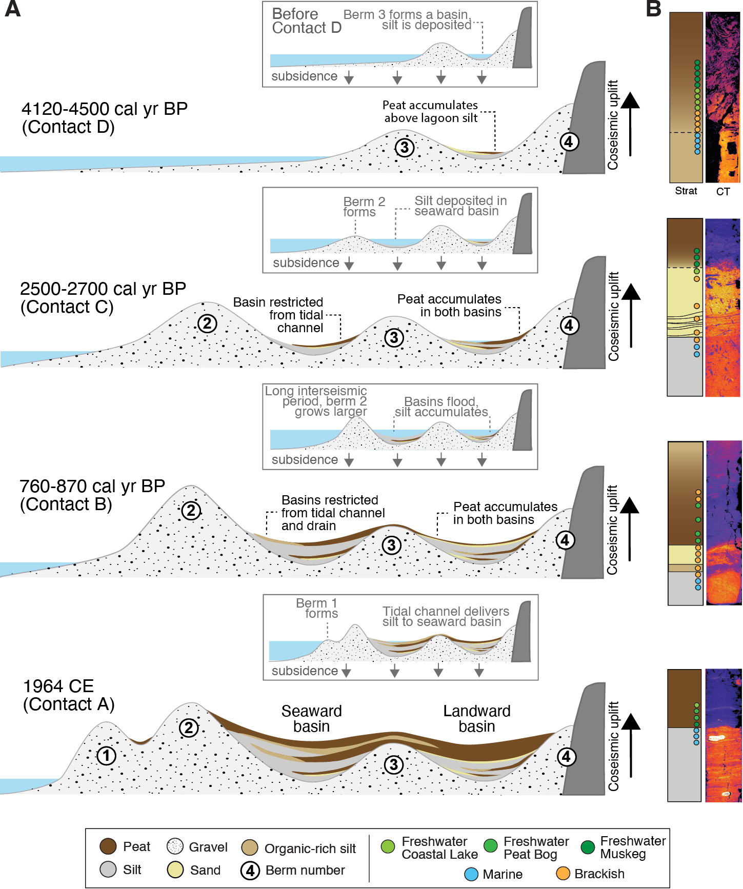Figure 2: (A) Inferred geomorphological change of the seaward and landward basins during and between major earthquakes (Contacts A-D) recorded at Hidden Lagoons, Montague Island, Alaska. (B) Representative stratigraphy and the corresponding Computed Tomography (CT) scan of each major contact are on the far right. Colored circles represent the transitions in diatom ecology at each sample location within the core. Figure and caption are modified from DePaolis et al. (2024).

Diatoms as indicators of coseismic uplift

During the 1964 CE Mw 9.2 Great Alaska Earthquake, the Patton Bay Splay Fault System, a steeply dipping fault system connected to the subduction zone at depth, was activated, contributing to the formation of local tsunamis, and causing significant (4–1 m) uplift of Montague Island in Prince William Sound (PWS; Plafker 1967). Aerial imagery from before and after the 1964 earthquake shows the gradual draining of coastal lagoons along its northwestern coast. DePaolis et al. (2024) investigated the coastal stratigraphy and diatom signature of the 1964 CE earthquake at Hidden Lagoons, Montague Island, and found a distinct silt-peat contact representing the draining of the coastal lagoon system. Diatom analysis showed the pre-earthquake lagoon system was a marine environment with direct tidal communication with the sea, while the post-earthquake diatoms indicated a gradual transition to a brackish, then freshwater lake, then freshwater bog environment, reflecting the gradual freshening and draining of the lagoon (Fig. 2). The ecological changes documented across the 1964 CE contact indicate >3 m of coseismic uplift, exceeding the amount of uplift expected from a subduction-zone-only rupture, and supporting the concurrent rupture of the splay fault system. Further investigation of the subsurface stratigraphy revealed an additional three sharp silt-peat contacts with diatoms displaying similar marine to freshwater ecological shifts across them. The older contacts overlap the timing of three of the seven independently constrained (Shennan and Hamilton 2006) prehistoric subduction zone earthquakes in PWS in 760–870, 2500–2700, and 4120–4500 yr BP. This suggests that the splay fault system may rupture jointly with the subduction zone every other, or every couple of, subduction-zone earthquakes, with a mean recurrence interval of ~1030 years. DePaolis et al. (2024) conclude that future hazard assessments should consider the potential risks of tsunamis associated with combined ruptures of subduction-zone splay fault systems, similar to those observed in historical and prehistoric events.

Diatoms have been used to quantify episodic postseismic uplift over the last 3000 years along the Kuril subduction zone in Japan, helping reconcile differences between long-term geologic uplift and shorter-term measurements of interseismic coastal subsidence. Despite no modern earthquake producing more than a few centimeters of uplift along coasts bordering the Kuril Trench, Sawai et al. (2004b) found stratigraphic and diatom evidence of episodic seismically triggered uplift of >1 m that repeatedly changed tidal flats into lowland forests on the island of Hokkaido, Japan, bordering the Kuril Trench. Sawai et al. (2004a, b) developed and applied a diatom-based transfer function to quantify the deformation following one of the events, a significant 17th-century earthquake and resulting tsunami, and found that fossilized diatom assemblages revealed a gradual, rather than sudden, transition from tidal flats into freshwater upland environments in the decades following the earthquake. Due to the gradual nature of the environmental transition, Sawai et al. (2004b) interpreted the 1.5 m of uplift to represent postseismic uplift of the coast. The results suggest that the earthquake ruptured the shallower parts of the subduction zone, triggering a tsunami, but did not produce coseismic uplift along the coast. Instead, Sawai et al. (2004b) attribute the uplift to postseismic slip deep on the plate boundary beneath the island on Hokkaido. Although it is unclear if the episodic uplift events documented by Sawai et al. (2004b) completely account for the long-term net uplift of marine terraces observed in Hokkaido, postseismic and possibly coseismic uplift from large and small earthquakes in the region certainly contribute to the long-term deformation of the coast.

affiliation

Department of Geosciences, Virginia Tech, Blacksburg, USA

contact

Tina Dura: tinadura@vt.edu

references

Atwater BF (1987) Science 236 (4804): 942-944

Briggs R et al. (2014) Geophys Res Lett 41(7): 2289-2296

DePaolis J et al. (2024) PhD Thesis, Virginia Tech, 137

Dura T et al. (2016) Earth-Sci Rev 152: 181-197

Dura T et al. (2017) Quat Sci Rev 175: 112-137

Hawkes A et al. (2011) Quat Sci Rev 30(3-4): 364-376

Klein E et al. (2017) Earth Planet Sci Lett 469: 123-134

Philibosian B, Meltzner AJ (2020) Quat Sci Rev 241: 106390

Plafker G et al. (1967) US Geol Surv Prof Pap: 1-42

Sawai Y et al. (2004a) Quat Sci Rev 23(23-24): 2467-2483

Sawai Y et al. (2004b) Science 306(5703): 1918-1920

Shennan I, Hamilton S (2006) Quat Sci Rev 25(1-2): 1-8

Sieh K et al. (2008) Science 322(5908): 1674-1678

Witter RC et al. (2016) Geophys Res Lett 43(1): 76-84

Past earthquakes have left geological imprints, and microfossil approaches using coastal sediments offer ways to constrain rupture characteristics over centennial to millennial timescales. New approaches may provide a means to reconstruct smaller earthquakes and improve our understanding of seismic hazards.

Great subduction-zone earthquakes (moment magnitude [Mw] >8) pose a significant threat to human populations, the environment and infrastructure, yet the spatial and temporal patterns of these hazards before the 20th century are often poorly constrained. Limited instrumental data (~100 years) offer only partial information on the potential magnitude, recurrence intervals and spatial variability of rupture area for past earthquakes due to infrequent occurrence (typically multi-centennial recurrence intervals) of great earthquakes. Impacts from the 2004 Sumatra and 2011 Japan earthquakes demonstrate the dangers of heavy reliance on temporally limited records (Dura et al. 2016). Great earthquakes can also trigger tsunamis that impact coastlines far from the rupture area and necessitate a better understanding of the hazard.

Paleoseismology, in general, can extend and constrain earthquake records beyond instrumental and historical data. Coastal sediments from low-energy environments contain valuable archives of past relative sea-level (RSL) changes and have been utilized globally (Dura et al. 2016). Sharp lithological contacts of alternating organic (peat) and minerogenic (silt) sediments often indicate abrupt vertical land-level changes associated with an earthquake. In Alaska, diatoms are the most common microfossil used to reconstruct RSL changes associated with great earthquakes due to their preservation potential, high abundance and ecological niches with respect to elevation within the tidal frame.

Use of diatoms in Alaskan paleoseismology

Alaska has played a pioneering role in our understanding of plate tectonics with the demonstration via multiple lines of evidence that the Mw 9.2 1964 CE earthquake was caused by a megathrust (e.g. Plafker 1965). Observations of land-level changes during this earthquake provided a framework for subduction-zone paleoseismology both in Alaska and globally. Initial studies focused on radiocarbon dating to understand the chronology of past events and used plants and lithology to estimate the magnitude of deformation (e.g. Combellick 1991). However, such approaches have limited vertical resolution with errors typically >0.5 m and, therefore, limit the ability to differentiate between different magnitudes of events. One approach to increasing the precision is to utilize microfossils such as diatoms (e.g. Hemphill-Haley 1995).

Diatoms are a group of photosynthetic, single-celled algae that are highly resistant to degradation due to their siliceous valves, allowing them to be incorporated into coastal sedimentary sequences, and preserved. Individual diatom taxa possess optima and tolerances to various environmental factors such as temperature, salinity and pH, making them highly sensitive to environmental change. The use of diatoms within Alaskan paleoseismology began through research conducted by Shennan et al. (1999) who examined the utility of diatoms to reconstruct the magnitude of land-level change at Girdwood. Since then, diatoms have been the most commonly utilized microfossil in Alaskan paleoseismology. Diatoms can be used in paleotsunami identification, with common characteristics of tsunami deposits including mixtures of fresh, brackish and marine diatoms (e.g. Fig. 1c), as well as broken and abraded valves (e.g. Dura et al. 2016; Hemphill-Haley 1995).

Paleoseismic evidence from coastal sediments currently provides a good understanding of great earthquakes in south-central Alaska, with records of approximately seven great earthquakes in the past 4000 years and 10 in the last 6000 years (Shennan et al. 2014). However, absolute correlations between sites are limited by uncertainties in radiocarbon chronologies (Barclay et al. 2024). Detailed diatom studies in this region from Cook Inlet, Cape Suckling and Cape Yakataga reveal two additional great earthquakes, in addition to the 1964 CE event, radiocarbon-dated to ~900 and ~1500 cal yr BP (Shennan et al. 2009, 2014). At the stratigraphic contact (peat-silt), diatoms display an increased abundance of marine taxa, indicating coseismic subsidence (Fig. 1b-c).

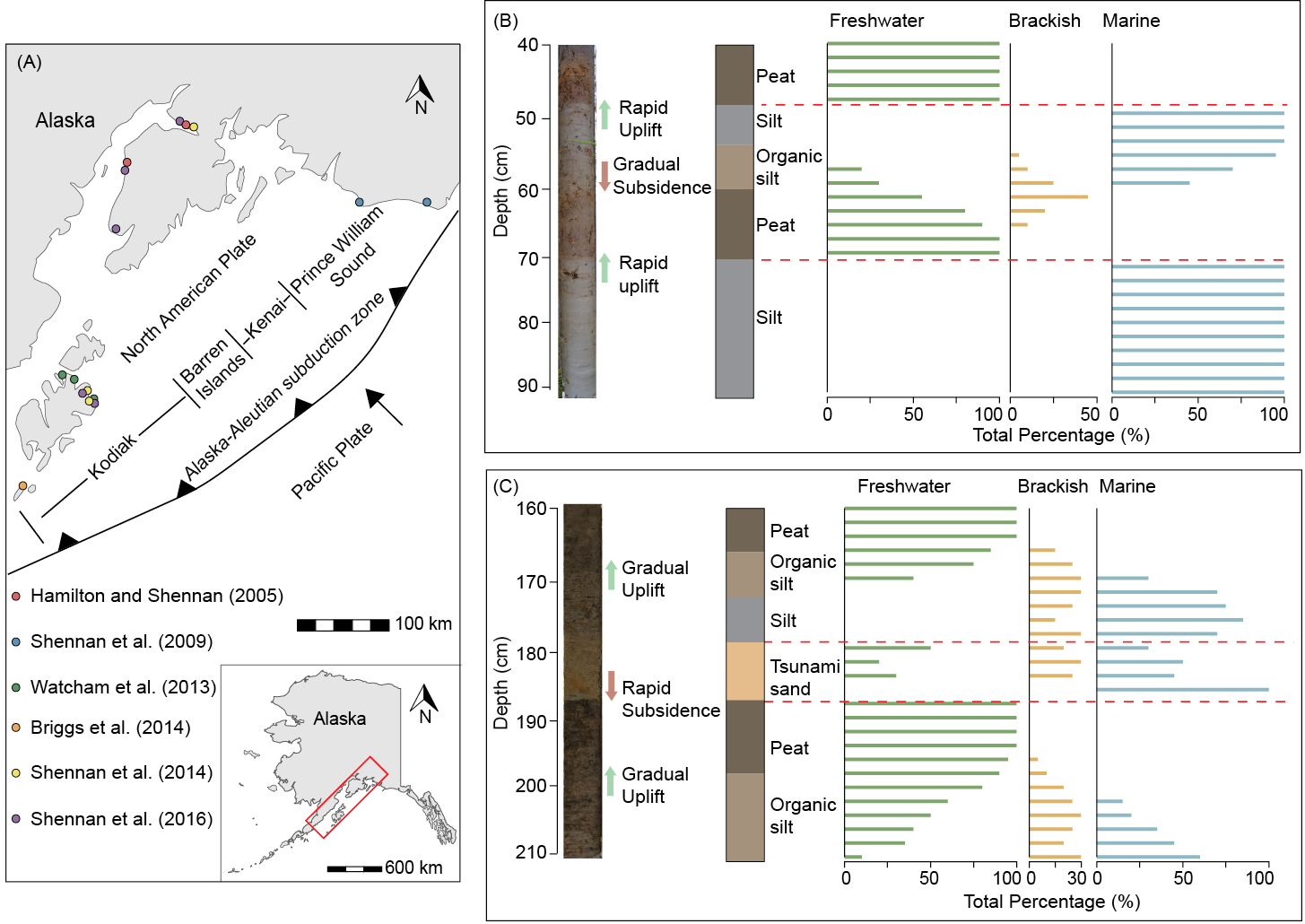Figure 1: (A) Location of Alaskan diatom research discussed within this article. For detailed information on diatom analysis for each site see the reference list. (B) Schematic showing simplified stratigraphy and theoretical diatom assemblages representing coseismic uplift and gradual interseismic subsidence. Photo credit: Dr. Rich Briggs. (C) Schematic showing simplified stratigraphy and theoretical diatom assemblages representing coseismic subsidence, a tsunami deposit and gradual interseismic uplift.

At the southwestern termination of the 1964 CE rupture, diatom analysis has also documented evidence of both uplift and subsidence at Sitkinak Island with five instances of vertical land-level motion over ~1200 years (Briggs et al. 2014). For example, coseismic subsidence is recorded in 1964 CE where diatom taxa show a shift from a freshwater and brackish assemblage to a brackish and marine assemblage. This is interpreted as indicative of the arrest of rupture at, or near, the island. In contrast, coseismic uplift, potentially related to a historically documented earthquake in 1788 CE, is identifiable by a change from a marine-dominated to freshwater-dominated assemblage. This variability in uplift and subsidence is also found for three older earthquakes. This finding of mixed uplift and subsidence suggests that rupture boundaries in the Alaskan–Aleutian subduction zone are not persistent. Similar conclusions regarding rupture variability were reached by Shennan et al. (2014) who, utilizing diatoms, inferred the possibility of both multi-section (rupture spanning the Kodiak section) and at least one other section (e.g. at 1964 CE) and single section (Individual section rupture where only the Kodiak section ruptured e.g. at 1440–1620 CE) ruptures. These results suggest shorter recurrence intervals within the Kodiak section, impacting hazard analysis.

Application of transfer functions

In paleoseismology, transfer functions quantify the relationship between modern diatom taxa and elevation. They can produce precise estimates of RSL change and have been tested against known amounts of subsidence, and shown to produce accurate results (e.g. Hamilton and Shennan 2005). The known contemporary relationship between modern diatom taxa and elevation (modern training set) can be applied to fossil assemblages within coastal stratigraphic sequences, to calculate the RSL changes throughout an earthquake cycle (Dura et al. 2016). However, diatom assemblages are very diverse and can result in challenges where the fossil diatom assemblage is not well represented in the modern training set; a no-modern analog situation (Watcham et al. 2013). When this occurs, quantitative reconstructions may not be reliable. Regional modern diatom datasets are more appropriate given the high diversity of diatom assemblages. They encompass modern taxa from a wide range of intertidal environments providing analogs for fossil diatom assemblages (Watcham et al. 2013). Further, Watcham et al. (2013) demonstrated that regional modern training sets with good modern analogs most closely matched observed subsidence when available.

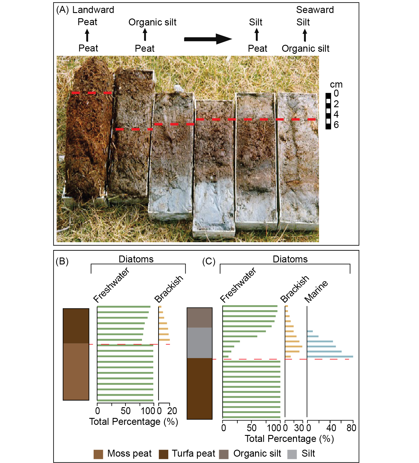Figure 2: (A) Sediment cores from near the city of Kenai demonstrating how the peat-silt subsidence contact from the great Mw 9.2 1964 CE earthquake (red dashed line) can be traced landward (from right to left) until the subsidence is expressed as a peat-to-peat contact. Photo credit: Prof. Ian Shennan. (B) Theoretical diatom assemblage for a peat-peat couplet. (C) Theoretical diatom assemblage for a peat-silt couplet.

Future directions

The methods used to study and identify great earthquakes within paleorecords are well-established. However, there remains a significant gap in our knowledge of the detection limit for smaller earthquakes. In November 2018 a Mw 7.1 earthquake occurred near Anchorage and produced land-level changes ranging from +2 to -5 cm (West et al. 2020), lying below our current estimates for detection within coastal sediments (0.1–0.2 m; Shennan et al. 2016). This earthquake had significant impacts on society, emphasizing the importance of a better understanding of the recurrence intervals of smaller earthquakes. Therefore, improving our understanding about the range of earthquake sizes which can be identified in coastal sediments is an important research objective.

Detection limits of coastal sediments are dependent on the tidal range, stratigraphy and choice of transfer function. Current criteria used to identify land-level change in coastal sediments rely heavily on clear and abrupt changes in sediment stratigraphy (peat-silt or silt-peat couplets) indicative of larger changes in RSL. However, the long interval between the penultimate earthquake, (1169–1189 CE; Barclay et al. 2024) and the great 1964 CE earthquake may require either significant strain to be carried to a future great earthquake, or to have been released by aseismic creep (steady fault movement generally without an associated earthquake), or smaller earthquakes in the intervening time period (Barclay et al. 2024). Diatom assemblages at Kenai and Shuyak Island identify coseismic subsidence associated with the 1964 CE earthquake within peat-peat couplets that are associated with the most precise transfer function estimates (Fig. 2a-c; Hamilton and Shennan 2005; Shennan et al. 2018; Watcham et al. 2013). Identifying peat-peat couplets associated with land-level change opens the possibility for detecting smaller earthquakes in coastal sediment sequences and is a topic of current and future research. New data generated from peat-peat couplets could also be correlated to recent lake paleoseismology research in south-central Alaska (e.g. Praet et al. 2017). The combination of these two techniques would allow for an integrated investigation into paleoseismic events.

affiliation

Department of Geography, University of Durham, UK

contact

Grace F. Summers: grace.f.summers@durham.ac.uk

references

Barclay DJ et al. (2024) Quat Sci Adv 13: 100142

Briggs RW et al. (2014) Geophys Res Lett 41: 2289-2296

Combellick RA (1991) DGGS Report of Investigations 112: 1-52

Dura T et al. (2016) Earth-Sci Rev 152: 181-197

Hamilton S, Shennan I (2005) Quat Sci Rev 24: 1479-1498

Hemphill-Haley E (1995) GSA Bulletin 107: 367-378

Plafker G (1965) Science 148: 1675-1687

Praet N et al. (2017) Mar Geol 384: 103-119

Shennan I et al. (1999) Quat Int 60: 55-73

Shennan I et al. (2009) Quat Sci Rev 28: 7-13

Shennan I et al. (2014) Geology 42: 687-690

Shennan I et al. (2016) Quat Sci Rev 150: 1-30

Shennan I et al. (2018) Quat Sci Rev 201: 380-395

Watcham EP et al. (2013) Quat Sci Rev 28: 165-179

West ME et al. (2020) Seis Res Lett 91: 66-84

Intertidal corals (microatolls) preserve evidence of past uplift or subsidence with annual precision. Microatoll records are particularly useful along subduction zones, and can reveal past earthquake ruptures at a level of detail that is ordinarily limited to the instrumental era.

The need for high-precision, widely distributed paleoseismic data

Decades of research have led to the realization that earthquake recurrence is complex, but nevertheless often follows a recognizable pattern (Philibosian and Meltzner 2020). Common patterns include rupture cascades (series of earthquakes on neighboring fault sections) and superimposed cycles (two or more neighboring fault sections with different recurrence intervals). To determine the types of recurrence patterns exhibited by a particular fault, it is necessary to establish details of past ruptures –timing, rupture extent, amount of fault slip –over several earthquake cycles. The required level of detail can be achieved only by using techniques with high temporal and spatial precision, as well as a wide distribution of study sites. The coral-microatoll technique, while limited in its applicability by the occurrence of reef-building corals above faults producing vertical movement, is perhaps the most precise among geologic-paleoseismic techniques.

The microatoll technique

The upward growth of corals in the intertidal zone is limited by relative sea level (RSL), as corals cannot survive for long out of the water. Reef-building coral species that grow radially outward generally form roughly hemispherical colonies underwater, but in the intertidal zone typically produce a colony with a flat, dead top, surrounded by a ring of living tissue that extends below the water.

The term "microatoll" was coined for these specimens based on their resemblance to ring-shaped coral reef atoll islands. As a microatoll grows outward, the height of the living outer ring responds to changes in RSL. Thus, the upper surfaces of microatolls record RSL over the lifetime of the colony, which in some species can reach hundreds of years. Furthermore, microatolls can be preserved in or near the intertidal zone for hundreds, or even thousands, of years after they die. Most coral species produce annual density bands analogous to tree rings. This combination of characteristics allows records of RSL to be reconstructed with annual precision over centuries, or millennia. Absolute ages of corals that died in the past are still limited by the precision of radiometric dating, but uranium-thorium disequilibrium dating can be used on corals, potentially yielding ages with uncertainties of less than a decade. Furthermore, the relative timing of events (annual precision) within a given coral record is not affected by absolute dating uncertainties.

Coral microatolls are sampled by cutting a radial slice, obtaining an X-ray image of the slice to reveal the annual bands, and measuring the growth height of each band (Fig. 1). Large, sudden height changes can be interpreted as earthquakes, whereas gradual trends in growth height over time record interseismic behavior. However, there are several interpretive steps between coral growth height and tectonic uplift or subsidence. The relationship between coral upward growth and RSL change is asymmetric, as a drop in sea level will cause the upper part of the coral to die within days, but a rise in sea level will usually leave an intertidal coral within its depth range, simply providing space for the coral to grow. This response takes years to be recorded (Fig. 2). In combination with the noise generated by interannual oceanographic fluctuations in sea level (such as those associated with the El Niño – Southern Oscillation), this means that gradual changes in RSL derived from microatoll records are often inaccurate unless averaged over a decade or more (as in Fig. 1d).

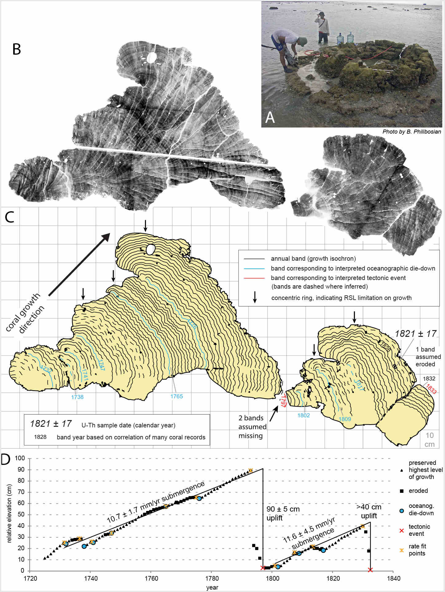Figure 1: Example microatoll interpretation (modified from Philibosian et al. 2014; Philibosian 2024). (A) A microatoll from which a radial slice is being cut with a hydraulic chainsaw. (B) X-ray image of the collected slice showing annual banding. (C) Interpreted microatoll cross-section. (D) Plot of annual coral growth height with measured uplifts and submergence rates estimated by linear fits to points preceding die-downs. This microatoll recorded two earthquakes 36 years apart; others have similarly recorded doublets separated by as little as four years (e.g. Philibosian et al. 2017).

Finally, to isolate tectonic uplift or subsidence, all other signals (most significantly eustatic sea-level change) must be removed from the RSL record (see Philibosian 2024). For sudden uplift or subsidence events (as often occur during earthquakes), the nontectonic contributions are generally negligible, but their impact can be more significant on estimates of gradual interseismic motion. Fortunately, most of the other potential signals affect large regions equally, such that any differences in RSL trend between nearby sites (up to a few hundred kilometers apart) can confidently be attributed to active tectonics.

In regions where coral microatolls are plentiful, numerous study sites can be fairly easily established over a broad area (Philibosian 2024). Whereas the specialized equipment and logistics for sampling microatolls are expensive, there are significant economies of scale that many other paleoseismic techniques (such as trenching) do not have.

Past and current applications

The coral-microatoll technique has long been used in paleoclimate studies (beginning with Scoffin and Stoddart 1978), and has since been applied and further tailored to earthquake research beginning with Taylor et al. (1987), but primarily in the 21st century. Thus far, the most extensive and successful use in an active tectonic context has been to establish the history of uplift and subsidence during and between earthquakes along the Sumatran Sunda Megathrust. The majority of the now-known best practices were established over the course of the Sumatran tectonic studies (see Meltzner and Woodroffe (2015) and Philibosian (2024) for details). These microatoll studies enabled multiple cycles of paleoearthquakes to be examined in unprecedented detail, including disambiguating individual events that occurred only a few years apart, and estimating rupture extent and slip magnitude for each event.

The Sumatran microatoll records have illuminated many hitherto underappreciated aspects of fault behavior, such as persistent rupture segmentation (e.g. Meltzner et al. 2012), complex earthquake recurrence cycles (Philibosian et al. 2012; Philibosian et al. 2017; Sieh et al. 2008), years-long slow-slip events (Tsang et al. 2015b), and variable strain accumulation over time (e.g. Meltzner et al. 2015; Philibosian et al. 2014; Tsang et al. 2015a).

The microatoll technique is gradually spreading to other tropical active-tectonic study areas, having been applied with varying degrees of success to subduction paleoseismology and paleogeodesy along the northernmost Sunda (Arakan) margin, the Solomon Islands, the Lesser Antilles, and the Ryukyu Arc, with nascent application in the Philippines. Microatolls have also served as vital recorders of uplift and subsidence during recent subduction earthquakes in Vanuatu and the Solomon Islands, as well as those along the Sumatran Sunda Megathrust. They have additionally been applied in an oblique strike-slip environment to measure vertical motion during the 2010 Haiti earthquake. Philibosian (in press) includes a complete current list of publications that have used coral microatolls in active tectonic studies.

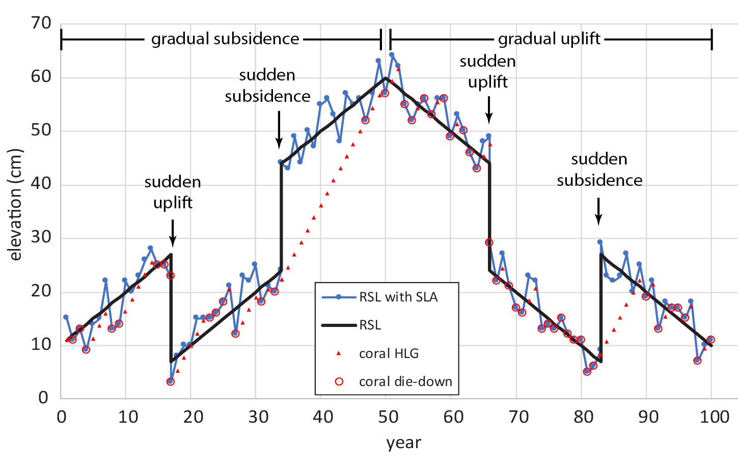Figure 2: Synthetic illustrative RSL history and resultant microatoll growth record (modified from Philibosian 2024). Black line shows RSL history with steady 1 cm/yr submergence over the first 50 years and equivalent emergence over the second 50 years, with sudden 20-cm emergence and submergence events during each period. Blue line with markers shows the same RSL curve with random ±5 cm interannual sea-level anomaly (SLA) fluctuation added. Red markers show response of a coral with 2.3 cm/yr upward growth rate; triangles indicate years in which height is limited by growth rate (highest level of growth, HLG) and circles show years when it is limited by sea level (die-downs).

Successful coral-microatoll studies ultimately provide maps of tectonic vertical motion with annual precision. This precision allows individual earthquakes that occurred only a few years apart to be distinguished in the geologic record, and demonstrates that no earthquakes producing significant uplift or subsidence occurred during parts of the record that lack sudden RSL changes. For each individual earthquake rupture, the distribution of uplift and subsidence can be modeled to obtain the rupture extent and fault-slip distribution, using the same procedures as would be done for any other type of surface-deformation measurement. Similarly, gradual interseismic vertical motion can be modeled to estimate the distribution of fault coupling and concomitant strain accumulation.

Obtaining such precise characteristics of individual paleoearthquakes is vital for assessing fault behavior, including the persistence of rupture segmentation, recurrence patterns, and similarity of successive events; key issues in both fault mechanics and hazard assessment. The coral-microatoll technique may be a useful component for any study involving active tectonic uplift or subsidence along coastlines where corals grow.

ACKNOWLEDGEMENTS

I thank the editors for the invitation to contribute this article, and Richard Briggs as well as the editors for helpful reviews.

affiliations

U.S. Geological Survey Earthquake Science Center, Moffett Field, California, USA

contact

Belle Philibosian: bphilibosian@usgs.gov

references

Meltzner AJ, Woodroffe CD (2015) In: Shennan I, Long AJ, Horton BP (Eds) Handbook of Sea-Level Research. Wiley

Meltzner AJ et al. (2012) J Geophys Res 117: Article B04405

Meltzner AJ et al. (2015) Quat Sci Rev 122: 258-281

Philibosian B (in press) In: Elliott AJ, Grützner C (Eds) Understanding Past Earthquakes. Springer-Nature

Philibosian B, Meltzner AJ (2020) Quaternary Science Reviews 241: 106390

Philibosian B et al. (2012) J Geophys Res 117: B05401

Philibosian B et al. (2014) J Geophys Res 119: 7258-7287

Philibosian B et al. (2017) J Geophys Res Solid Earth 122: 642-676

Scoffin TP, Stoddart DR (1978) Philos Trans R Soc London Ser B 284: 99-122

Sieh K et al. (2008) Science 322: 1674-1678

Taylor FW et al. (1987) J Geophys Res 92: 4905-4933

Tsang LLH et al. (2015a) Geophys Res Lett 42: 10585-10594

Tsang LLH et al. (2015b) Geophys Res Lett 42: 6630-6638