PAGES Magazine articles

Paleoclimate data are essential to gauge the magnitude and the speed of change in greenhouse gas concentrations, ocean acidification, and climate. These parameters co-determine the anthropogenic impacts on natural and socioeconomic systems and their capabilities to adapt.

Concentrations of the three major anthropogenic greenhouse gases were much smaller during at least the last 800 ka than modern and projected concentrations. The ice core record reveals that the average rate of increase in CO2 and the radiative forcing from the combination of CO2, CH4, and N2O occurred by more than an order of magnitude faster during the Industrial Era than during any comparable period of at least the past 16 ka (Joos and Spahni 2008). This implies that current global climate change and ocean acidification is progressing at a speed that is unprecedented at least since the agricultural period.

Ice, terrestrial and oceanic records reveal huge changes in climate during glacial periods on the decadal time scale (Jansen et al. 2007). These are linked to major reorganizations of the oceanic and atmospheric circulations, including a stop and go of the poleward Atlantic heat transport and shifts in the rain belt of the Inter Tropical Convergence Zone (ITCZ). These ”Dansgaard-Oeschger” and related Southern Hemisphere climate swings demonstrate that the climate system can switch into new states within decades – a potential for unpleasant future surprise.

Surprisingly, variations in atmospheric CO2 remained quite small during Dansgaard-Oeschger events. This indicates a certain insensitivity of atmospheric CO2 to shifts in the ITCZ, changes in the ocean’s overturning circulation, and abrupt warming of the boreal zone. Related variations in N2O and CH4 are substantial (Schilt et al. 2010), but the resulting radiative forcing is several times smaller than current anthropogenic forcing. Greenhouse gas concentrations react to climate change and amplify it, but the data may also indicate that such an amplification of man-made climate change may remain moderate compared to anthropogenic emissions. This is in line with results from Earth System Models and probabilistic analyses of the last millennium temperature and CO2 records (Frank et al. 2010).

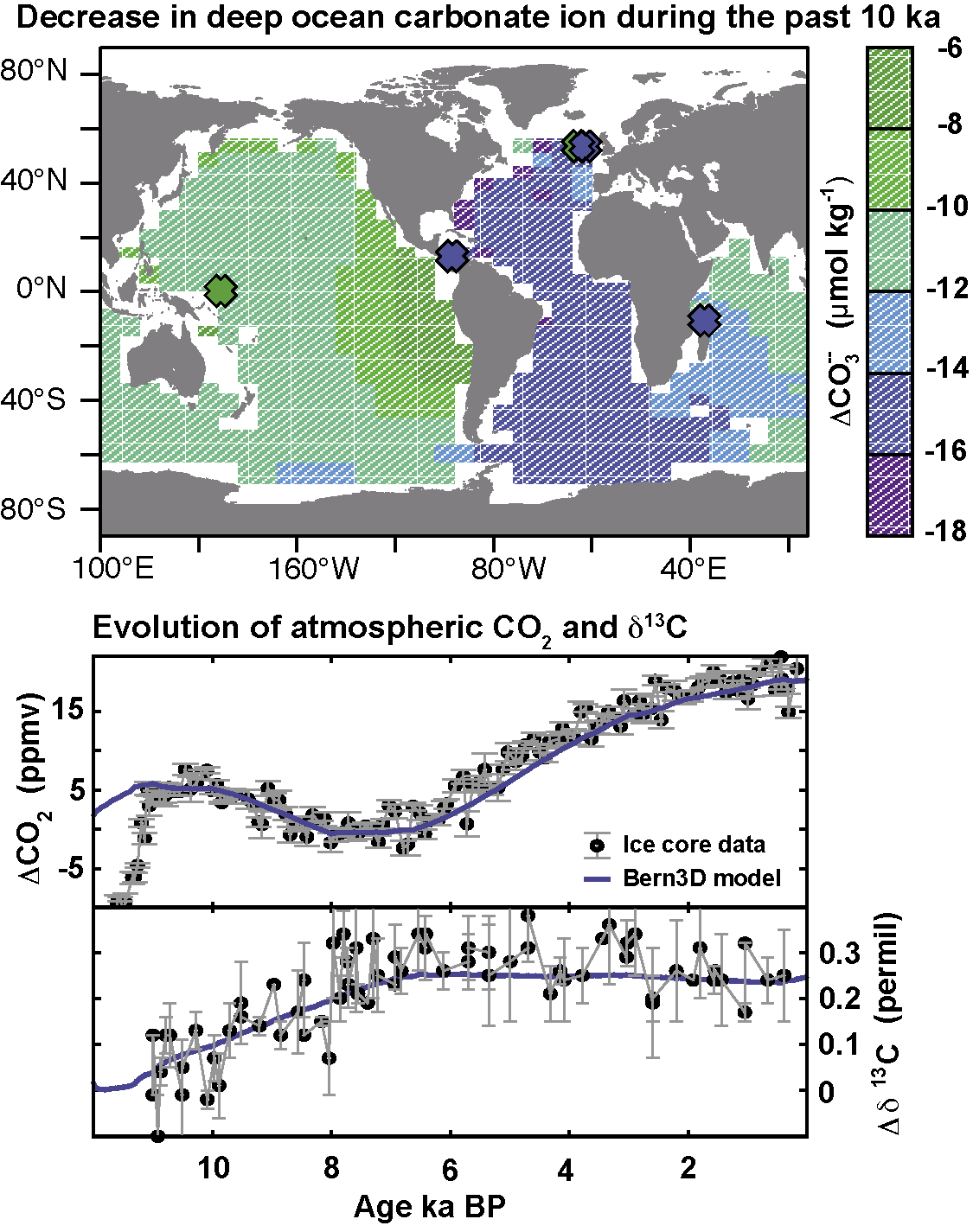
Figure 1: Evolution of atmospheric CO2 and δ13C of atmospheric CO2 (lower panel) and changes in deep ocean carbonate ion concentration (μmol kg-1) over the last 10 ka (upper panel). Proxy data are shown by circles and crosses, and results from the Bern3D model by blue lines and color contours (after Menviel and Joos 2012).

Theories and Earth system models must undergo the reality check to quantitatively explain the observations. For example, reconstructed and simulated spatio-temporal evolution of C-cycle parameters during the last 11 ka (Fig. 1) provide evidence that the millennial-scale CO2 variations during the Holocene are primarily governed by natural processes (Menviel and Joos 2012), in contrast to previous claims of anthropogenic causes.

Paleoscience allows us to test hypothesis. Can we mitigate the man-made CO2 increase by stimulating marine productivity and promoting an ocean carbon sink by artificial iron fertilization? Paleodata (Röthlisberger et al. 2004) and modeling suggest that we can’t – past variations in aeolian iron input are not coupled to large atmospheric CO2 changes.

Warming might set carbon free from permafrost and peat or CH4 currently caged in clathrates in sediments, which would in turn amplify global warming and ocean acidification. However, soil, atmospheric CO2 and carbon isotope data suggest a carbon sink, and not a source, in peatlands during periods of past warming (Yu 2010). Likewise, ice core data show no extraordinarily large CH4 variations nor supporting isotopic signatures (Bock et al. 2010) for thermodynamic conditions potentially favoring CH4 release from clathrates, i.e. during periods of rapid warming and sea level rise.

Yet, it is not always clear to which extent a comparison of the past with man-made climate change is viable. We need to improve our mechanistic understanding of the underlying processes to better assess the risk of ongoing greenhouse gas release and associated climate amplification and feedbacks in order to better guide emission mitigation and climate adaptation efforts. Paleoresearch, offering unique access to time scales and complex climate variations neither covered in the instrumental records nor accessible by laboratory studies, is the key to reach this policy-relevant goal, but its potential has barely been exploited.

selected references

Full reference list online under: http://pastglobalchanges.org/products/newsletters/ref2012_1.pdf

Frank DC et al. (2010) Nature 463: 527-530

Menviel L and Joos F (2012) Paleoceanography 27(1), doi: 10.1029/2011PA002224

Röthlisberger R et al. (2004) Geophysical Research Letters 31, doi: 10.1029/2004GL020338

Schilt A et al. (2010) Quaternary Science Reviews 29(1-2): 182-192

Yu Z (2010) The Holocene 21(5): 761-774

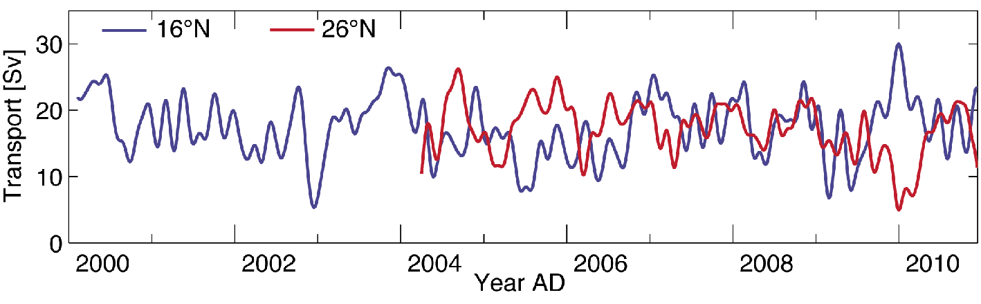
Figure 1: Southward Deepwater Transport at 16°N (blue line) and Strength of Meridional Overturning at 26°N (red line) for the period 2000-2010 AD.

Earth’s oceans undergo a relentless churning as water responds to the interplay of temperature, salinity and prevalent winds. In the Atlantic Ocean, roughly 18 Sv1 of warm, saline near-surface water is carried northward by the Gulf Stream/North Atlantic Current system (Cunningham et al. 2007). An equivalent amount of cold, deep water from the Nordic and Labrador Seas is guided by topography to the Southern Ocean. Here, it returns to the upper ocean more slowly via the mixing of deeper and shallower waters and/or the upwelling of deeper water in response to the strong westerly winds. This global-scale Meridional Overturning Circulation (MOC) is responsible for the observed temperature contrast of 15°C at low-latitudes in the Atlantic between the upper ocean and the deep ocean. In contrast, the absence of deep water formation in the Northern Pacific and Indian Oceans means that oceanic northward heat transport is significantly less than in the North Atlantic (Lumpkin and Speer 2007).

In its fourth assessment report the Intergovernmental Panel of Climate Change considers it “very likely” that the MOC will have gradually slowed by the end of the 21st century as a consequence of global warming. Climate model projections predict a slowdown between 0 and 50% by the year 2100, although complete shutdown is considered “unlikely” for this time horizon. The reasons for the slowdown include factors that impede deep-water formation – warming of surface waters and salinity reduction at high latitudes due to the melting of continental ice sheets and the intensification of the hydrological cycle. Uncertainties regarding the freshwater fluxes and the locations of deep-water formation at high latitudes are the primary causes of the large uncertainties in the model projections.

Future changes to the MOC will also be determined by changes in the mechanisms leading to the upwelling of warmer waters. Winds have intensified by 30% over the Southern Ocean during the second half of the last century (Huang et al. 2006), possibly due to decreasing stratospheric ozone concentrations. This trend is expected to prevail until 2100 (Shindell and Schmidt 2004). Beyond the end of this century, in what will be a different climate, upwelling in the Southern Ocean might gain in importance relative to sinking in the North Atlantic. Other long-term influences on the overturning in the North Atlantic Ocean are related to increased surface saltwater exchanges between the Indian and South Atlantic Oceans in the Agulhas Current System.

At present, there is no convincing observational evidence for a long-term weakening of the Atlantic MOC. This absence of evidence should not be mistaken as evidence of absence of a slowdown, especially when there is a lack of adequate long-term and sustained monitoring. Discontinuous historic observations do not capture the large intraseasonal-to-interannual variations, thereby reducing the reliability of the projections of the long-term changes in the MOC. Continuous measurements spanning the past decade or so are not indicative of a “strong” MOC decline. But on decadal time scales, natural variations have considerably larger amplitudes than the anthropogenic signature (on the order of 0.5 Sv per decade). Thus, observations sustained over several decades are required to distinguish between natural and anthropogenic changes.

Monitoring of the MOC has improved since the beginning of this century (Kanzow et al. 2010; Send et al., in press). Methods include those based on ocean state estimates and those using numerical models to identify observable variables (indices) that correlate well with the MOC strength in the models. Careful validation against the existing direct observations is now required to establish the robustness of state-estimate-based and index-based changes to the MOC. In principle these methods could also be applied to paleo-oceanographic proxies, to open a window to ocean-induced changes in past climate.

11 Sv= 106 m3s-1, unit for volumetric transport. For comparison, the Amazon River discharge in the Atlantic is about 0.2 Sv

A foundational geological concept that is attributed to James Hutton, the principle of “uniformitarianism”, holds that the present is the key to the past. However, the observable present cannot capture the full dynamic range of the climate system, and it is therefore to the past that we must turn for a broader perspective on climate change. What is clear from the geological record is that the large-scale ocean circulation is not immutable; it has changed repeatedly in the past and in intimate connection with global and regional climate shifts. What is generally less clear, is exactly what aspect of the ocean circulation has changed in each instance (mass transport, interior mixing rates, transport pathways?), to what degree, and why. These ambiguities arise from two principle challenges in paleoceanography: first, the challenge of inferring hydrographic observations from ”proxies”; and second, the challenge of inferring the ocean’s large-scale circulation from sparse hydrographic observations, often with highly uncertain age-control. These difficulties become exacerbated when attempting to reconstruct analogues of the relatively subtle, high frequency or seasonally expressed changes in the ocean circulation that are likely to be most relevant to climate change in the decades to come.

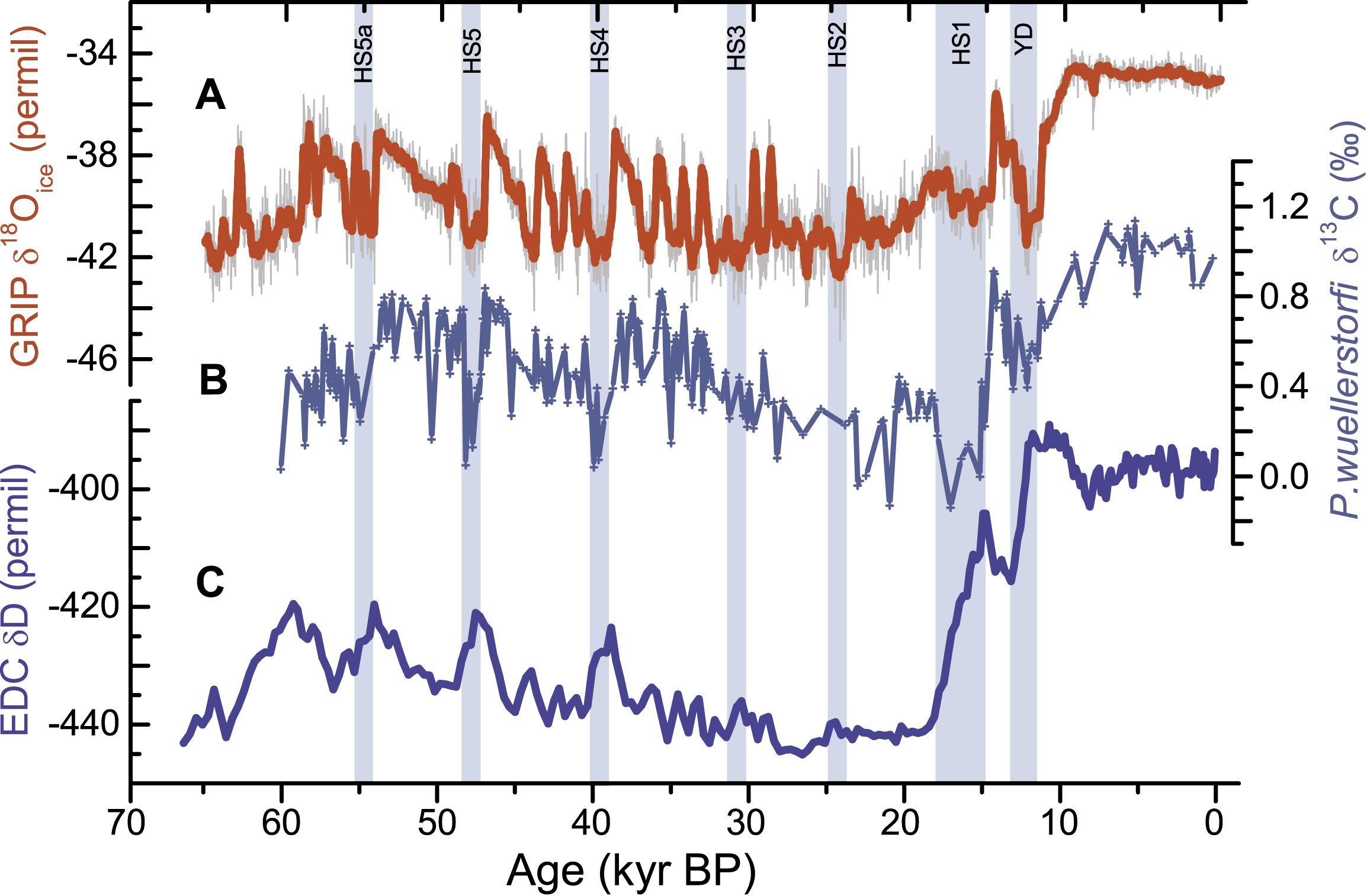
Figure 1: Changes in the ocean-climate system over the past 60 ka, showing climate anomalies over Greenland (A) and Antarctica (C) (Lemieux-Dudon et al., 2010) compared with evidence for ocean circulation changes from the deep Northeast Atlantic (B) (Skinner et al. 2007). The evidence for circulation changes is derived from benthic foraminiferal stable carbon isotopes, which are interpreted here to represent primarily the preformed macro-nutrient content of deep waters, and therefore the relative dominance of northern- versus southern deep-waters in the deep North Atlantic. HS: Heinrich Stadial, YD: Younger Dryas.

Perhaps the most robust case study in past ocean-climate linkages comes from the last 60 ka. This time period has witnessed a succession of regional climate changes, with Greenland and the North Atlantic region exhibiting rapid warm/cold alternations in association with coupled but asynchronous changes in Antarctic temperature. The largest of these climatic perturbations also coincide with changes in the chemistry of waters filling the deep Atlantic (Fig. 1B). The latter are most easily attributed to shifts in the distribution of different water-masses, and therefore to changes in the ocean circulation; a view that is broadly consistent with some numerical model simulations (Ganopolski and Rahmstorf 2001; Liu et al. 2009).

The prevailing interpretation of the records shown in Figure 1 is that they represent the operation of a ”thermal bipolar seesaw”, resulting from changes in the ”effectiveness” of the Atlantic overturning circulation as a heat pump from southern to northern latitudes (Schmittner et al. 2003). The hypothesized trigger for these overturning perturbations is anomalous melt-water supply to the North Atlantic: i.e. ice-sheet or ice-shelf surges that may well have been climatically driven (Alvarez-Solas et al. 2010; Flückiger et al. 2006). Interestingly, the patterns and associations of these rapid ocean-climate changes appear to be consistent with an overturning circulation that is conditionally stable, and that may respond non-linearly to relatively subtle perturbations, depending on the prevailing climate/forcing conditions (Margari et al. 2009; Rahmstorf et al. 2005). Indeed, through their inter-hemispheric teleconnections and their inferred impact on the carbon cycle (Anderson et al. 2009), such non-linear shifts in the ocean circulation are thought to have played a key role in tipping global climate out of its glacial state ca. 15-20 ka ago (Barker et al. 2011). Once this happened, ocean-climate variability appears to have become more subdued. Although this suggests a relative stabilization of the ocean circulation under interglacial conditions, it does not imply the complete elimination of ocean-climate variability during the Holocene. Indeed, evidence exists for centennial to millennial perturbations during the Holocene that are likely to have dwarfed those recorded in the instrumental record.

What can these impressive, if incompletely understood, changes in the past ocean-climate system teach us? In general, they question the paradigm of the ocean circulation as a millennially sluggish flywheel in the climate system. They suggest a capacity to respond sensitively to, and in turn impact significantly on regional and global climate, possibly in a non-linear fashion and with important ramifications for the carbon cycle and the global energy budget. However, the past does not provide an easy template for the future. If the geological record is to inform more directly on the stability properties of our modern circulation and its immediate future, paleoceanographers will need to focus on past ocean-climate variability in increasingly fine detail, and with a particular emphasis on relatively warm climate conditions.

selected references

Full reference list online under: http://pastglobalchanges.org/products/newsletters/ref2012_1.pdf

Alvarez-Solas J et al. (2010) Nature Geoscience 3: 122-126

Anderson RF et al. (2009) Science 323: 1443-1448

Barker S et al. (2011) Science 334: 347-351

Margari V et al. (2009) Nature Geoscience 3(2): 127-131

Schmittner A et al. (2003) Quaternary Science Reviews 22: 659-671

The biological pump refers to a suite of biologically mediated processes that transport carbon from the ocean’s surface layer to its interior. Its efficiency depends on the balance between the rates of carbon photo-assimilation, export and mineralization. Our knowledge of the biological carbon pump relies on our mechanistic understanding of factors structuring phytoplankton distributions and marine food webs, and the associated biogeochemical cycles. To assess the extent to which the strength and the efficiency of this pump will change in the future, we need to know how these factors – light, nutrients and temperature – might change in a warmer ocean. Models coupling an ecosystem module to a global circulation model provide important tools for understanding the dynamics of the carbon pump and its response to warming. But as pointed out by Sarmiento et al. (2004), existing tools are still not mature enough to allow this.

The last decade has seen increasing awareness of the relationship between key phytoplankton groups and their pivotal role in the functioning of the biological carbon pump (e.g. Boyd et al. 2010). Until recently, the picture was of a simple subdivision between efficient carbon export via a diatom-copepod-fish linear food chain in nutrient-rich waters and retention of surface carbon in nutrient-poor waters via a microbial network initiated by the ubiquitous pico/nano phytoplankton (Chisholm 2000). This picture has been recently complicated by the recognition of two additional small-sized players – the calcifying coccolithophores and the nitrogen-fixing cyanobacteria. These have a competitive advantage over diatoms in warm, well-illuminated surface waters supplied with imbalanced inorganic nitrogen and phosphorus nutrients. Their participation in carbon export is indirect and involves either aggregation with calcium carbonate liths acting as ballast particles or the release of nitrogen that sustains the growth of concomitant diatoms, thereby triggering carbon export (Chen et al. 2011).

Figure 1: Summer conditions in the upper water layers of the Canadian Basin. The lower panel shows the physical water properties over the period 2004-2008, the upper the response of the plankton organisms during the same period. Figure modified from Li et al. 2009.

Ocean warming affects the pelagic ecosystem both directly and indirectly, by increasing temperature and stratification. The latter tend to favor the dominance of small phytoplankton (e.g. Falkowski and Oliver 2007; Li et al. 2009) over large cells such as diatoms (Fig. 1). The resulting photo-assimilated carbon benefits the heterotrophic microbial food web, whose activity is stimulated by the warmer temperature (Sarmento et al. 2010), increasing the rate of carbon mineralization. Small phytoplankton cells also have low sinking rates. The spreading of such cells anticipated with increased ocean stratification will decrease the overall capacity of the biological pump, but the extent remains uncertain (Barber 2007).

The prevalent view of the picophytoplankton carbon being totally remineralized in the surface waters has been recently challenged by data from the equatorial Pacific Ocean and Arabian Sea, which point to significant export of picophytoplankton-related carbon through indirect paths such as aggregation and fecal pellets (Richardson and Jackson 2007). The future latitudinal extent of coccolithophore blooms due to warming is unknown, however, particularly in light of the possible alteration of calcification rates by ocean acidification (Cermeño et al. 2008).

The potentially large ocean deoxygenation due to the increased temperature and stratification projected for a warmer ocean (Keeling et al. 2010) will have direct consequences for marine biota, but only an indirect effect on ocean productivity and nutrient and carbon cycling. An expansion of suboxic/anoxic conditions would increase the release of phosphate and iron from sediments while some reactive nitrogen would be eliminated by denitrification or anaerobic ammonia oxidation. The subsequent shift in the ocean nitrate-to-phosphate balance will affect the composition and productivity of marine organisms, notably diazotrophic cyanobacteria, with uncertain consequences for the efficiency of the biological pump.

On the whole, the smallest phytoplanktons seem to have a competitive advantage in a warmer ocean. In contrast, diatoms are at an advantage in surface waters with transient nutrient pulses. In particular, they will benefit in coastal regions from stronger wind-driven upwelling events that are expected from increased storm and frequency resulting from climate warming. Improving the evaluation of changes to the biological carbon pump via ocean models is currently hampered by several uncertainties on mechanisms controlling phytoplankton dominance and food-web structures. Also, many global circulation models remain coarse in resolution and don’t serve high frequency forcing. To be able to predict better the efficiency of the pump under future conditions, the complexity in biology needs to be matched with an appropriate complexity in the representation of the physical and chemical environment in ocean models.

references

Full reference list online under: http://pastglobalchanges.org/products/newsletters/ref2012_1.pdf

Boyd PW, Strzepek R, Fu F and Hutchins D (2010) Limnology and Oceanography 55(3): 1353-1376

Chen Y-L L, Tuo S-H and Chen H-Y (2011) Marine Ecology Process Series 421: 25-38

Keeling RF, Kortzinger A and Gruber N (2010) Annual Reviews of Marine Science 2: 199-229

Richardson TL and Jackson GA (2007) Science 315: 838-840

Sarmento H et al. (2010) Philosophical Transactions of the Royal Society B 365: 2137-2149

Changes in oceanic carbon storage have been hypothesized to be the cause of the ~100 ppm variations in atmospheric CO2 between glacials and interglacials (Sigman and Boyle 2000). If the ocean stores more carbon in colder than in warmer climates this implies that a positive feedback exists: as climate warms the ocean releases carbon, which increases atmospheric CO2 and amplifies the original warming. However, presently we don’t know how much ocean carbon storage changed in the past and why.

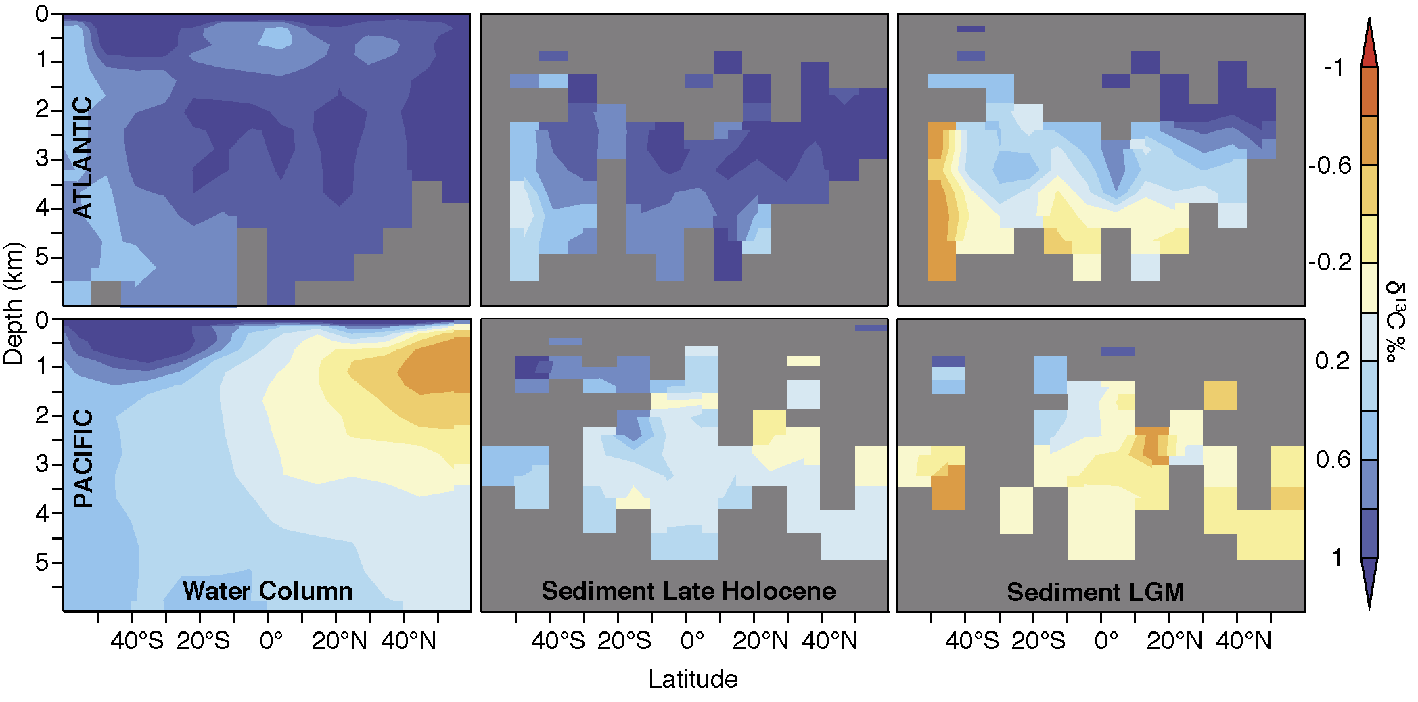
Figure 1: Latitude-depth distribution of zonally averaged δ13C in the Atlantic (top) and Pacific (bottom. Left: modern water-column measurements from WOCE and CLIVAR cruises (Schmittner et al., unpublished data). Middle: Late Holocene sediment data. Right: LGM sediment data. Sediment data from Hesse et al. (2011) and Matsumoto et al. (2002).

Carbon isotope data from Last Glacial Maximum (LGM, 19-22 ka) sediments indicate that more carbon was stored in the deepest ocean layers, particularly in the Atlantic (Fig. 1). δ13C is fractionated during carbon uptake by phytoplankton, which favors the light isotope 12C. Its distribution in the deep ocean is therefore determined to a large degree by the efficiency of the biological carbon pump, with lower values indicating more respired carbon.

In the modern ocean deep waters in the North Atlantic are high (+1‰) in δ13C and quite homogenous, corresponding to sinking of low nutrient, high oxygen surface waters. δ13C values are lower in the Southern Ocean (+0.5‰ ) and decrease towards the North Pacific (−0.6‰), reflecting today’s ocean’s oldest waters with high nutrients and carbon and low oxygen.

During the LGM, the deep Atlantic had much larger vertical gradients than today, δ13C values measured on microfossil shells of benthic foraminifera were up to 1‰ lower below 2-3 km depth, but similar above 2 km in the north (e.g. Curry and Oppo 2005). The deep Pacific Ocean was also higher in δ13C particularly in the south (Matsumoto et al. 2002). In contrast to the North Atlantic, however, the North Pacific did not exhibit larger vertical gradients. The coherent large-scale differences in δ13C suggest that biological carbon storage in the glacial ocean was most likely higher than today. But how much higher was it and why?

Biological, physical and chemical processes determine biological carbon storage in the ocean. It is likely that more than one process must be invoked to explain glacial to interglacial changes (Köhler et al. 2005). Increased solubility of CO2 in colder water explains less than 20 ppm of the full glacial-interglacial difference. The increase in the vertical gradient of δ13C in the Atlantic may require changes in the circulation such as a shoaling of the southward flowing deep waters or a change in the rate of northward flowing bottom waters. Furthermore, in a simple model of Bouttes et al. (2009) increased brine rejection from sea ice around Antarctica and its effect on deep ocean stratification lowered atmospheric CO2 by ~42 ppm, but the effect will need to be reproduced with more realistic models. Large changes in the contributions of northern versus southern sources to the global deep water can also change the efficiency of the biological pump (Martin 1990), but did not contribute much to the glacial-interglacial atmospheric CO2 changes.

The efficiency of plankton to use nitrate and phosphate may have been enhanced by more iron input to the surface ocean by higher dust deposition (Brovkin et al. 2007, estimate 37 ppm). A glacial dust plume from Patagonia may partly explain lower δ13C in South Atlantic bottom waters but the increase in aeolian iron input may have been counteracted by a decrease in sedimentary sources due to lower sea level (Moore and Braucher 2008). It is also possible that the biologically available (fixed) nitrogen inventory of the glacial ocean was overall higher than today because denitrification was lower due to higher dissolved oxygen concentrations in the colder glacial ocean and reduced continental shelf area due to the sea level drop. However, these processes have not been quantified yet with a realistic 3-dimensional model.

Some or all of the processes that controlled changes in the glacial-interglacial ocean carbon storage may also be important for our warming planet. Decreased CO2 solubility in a warming ocean will certainly occur. However, how important some of the other processes will be in the future is more uncertain. Better understanding of how and why ocean carbon storage varied in the past and in the future may now be possible due to coordinated international modeling projects and efforts to synthesize and increase the spatial coverage of paleoclimate data.

selected references

Full reference list online under: http://pastglobalchanges.org/products/newsletters/ref2012_1.pdf

Bouttes N, Roche DM and Paillard D (2009) Paleoceanography 24, doi: 10.1029/2008PA001707

Brovkin V, Ganopolski A, Archer D and Rahmstorf S (2007) Paleoceanography 22, doi: 10.1029/2006PA001380

Martin JH (1990) Paleoceanography 5(1): 1-13

Matsumoto K, Oba T, Lynch-Stieglitz J and Yamamoto H (2002) Quaternary Science Reviews 21: 1693-1704

Moore JK and Braucher O (2008) Biogeosciences 5: 631-656

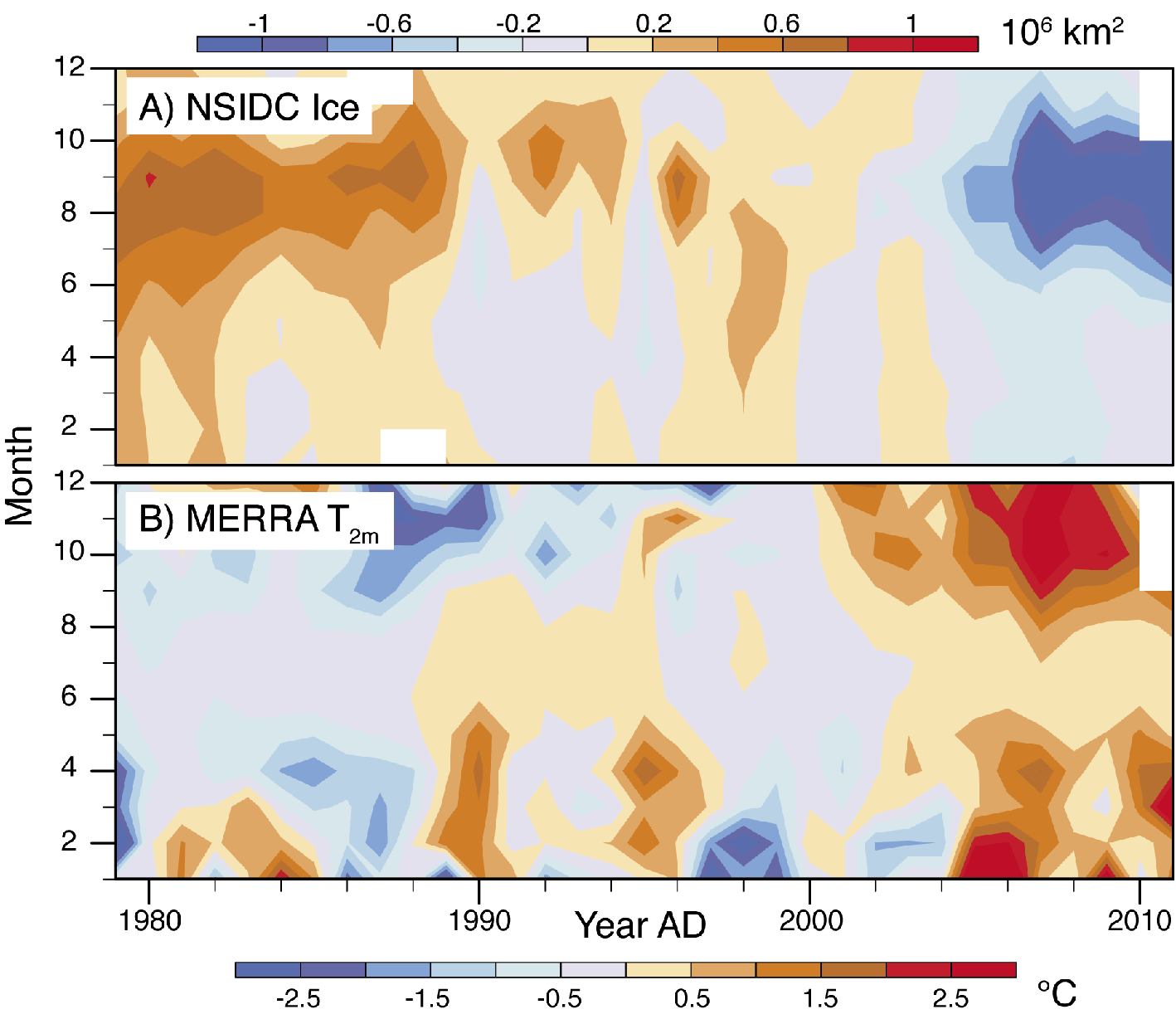
Figure 1: Time series by month (y-axis) and year (x-axis) of (top) anomalies in Arctic sea ice extent based on the satellite passive microwave record and (bottom) corresponding anomalies in 2-meter air temperate for the Arctic Ocean based on the NASA Modern Era Retrospective-Analysis for Research and Applications (MERRA). Anomalies are calculated with respect to the period 1979-2010.

It seems inevitable that the Arctic will lose its summer sea ice cover as air temperatures continue to rise in response to increased concentrations of atmospheric greenhouse gases. Over the last 33 years for which we have high quality records from satellite remote sensing, the September (end-of-summer) sea-ice extent has declined at a rate of 13% per decade. The five lowest September extents in the satellite record have all been in the past five years; average extent for this period represents a 35% reduction compared to conditions in the 1980s. Although there will likely be winter sea ice for centuries to come, the ice that forms in winter will be too thin to survive the summer melt season.

Emerging results from the latest generation of coupled global climate models indicate that essentially ice-free conditions (with some residual ice surviving in favored locations) could be realized as early as 2030. However, we may get to an essentially ice free Arctic Ocean, only to see temporary recovery. Modeling work argues for both decadal-scale periods of especially rapid ice loss in the future and periods of increasing ice extent. This implies that concern over a tipping point in ice thickness that, when crossed results in a rapid slide to an ice-free state, is likely unfounded.

Given that environmental impacts of ice loss will be realized well before one gets to a truly ice-free state, the year at which we first see a blue Arctic Ocean is not as important as when the bulk of the ice is gone. Some within-Arctic impacts of sea-ice loss are already here. This includes loss of species habitat, northward migration of marine species, and increased coastal erosion along the Beaufort Sea coasts and elsewhere due to increased wave action and thermal erosion of permafrost-rich coastal bluffs (Overeem et al. 2011). The observed greening of the Arctic coastal tundra, as determined from satellite measurements of photosynthetic activity, is at least in part a response to loss of the local chilling effect of coastal ice (Bhatt et al. 2010).

Simulations with the first generation of global climate models projected that as the climate system responds to an increased level of carbon dioxide, there would be an outsized warming of the Arctic compared to the globe as a whole (Manabe and Stouffer 1980), a phenomenon termed Arctic amplification. While a number of processes can lead to Arctic amplification, summer sea-ice loss is a major driver: as the ice retreats in summer, there are ever larger areas of open water that readily absorb solar radiation and add heat to the ocean mixed layer. When the sun sets in autumn, this heat is released upwards, warming the overlying atmosphere. Arctic amplification has emerged strongly over the past decade of anomalously low summer sea-ice conditions.

There is growing recognition that Arctic amplification, through altering the static stability of the atmosphere, water vapor content and horizontal temperature gradients, will influence the character of weather patterns within and beyond the Arctic. Observational evidence suggests that high-latitude atmospheric circulation is already responding to ice loss, and a variety of studies indicate that these effects will become more pronounced in the coming decades (Serreze and Barry 2011). At least one modeling study finds that the warming effects of sea-ice loss will extend far inland, contributing to warming of the tundra soil column, hastening permafrost thaw and the release of stored carbon to the atmosphere (Lawrence et al. 2008). In short, there seem to be many reasons why we should care about losing the summer Arctic sea-ice cover.

selected references

Full reference list online under: http://pastglobalchanges.org/products/newsletters/ref2012_1.pdf

Bhatt US et al. (2010) Earth Interactions 14: 1-20

Lawrence DM et al. (2008) Geophysical Research Letters 35, doi: 10.1029/2008GL033894

Manabe S and Stouffer RJ (1980) Journal of Geophysical Research 85: 5529-5554

Overeem I et al. (2011) Geophysical Resesearch Letters 38, doi: 10.1029/2011GL04681

Serreze MC and Barry RG (2011) Global and Planetary Change 77: 85-96

As Arctic sea ice is shrinking at an accelerating speed for the fourth decade in a row and summer ice extent numbers are falling well below the range of historical observations, much attention is placed on paleoclimatic reconstructions based on long-term time series. This situation necessitates a clear understanding of the nature and limitations of paleo records that can be employed in the Arctic Ocean. The most direct long-term records of sea-ice changes could be derived from seafloor sediments. Not surprisingly, Arctic paleoceanographic research is currently on the rise (Polyak and Jakobsson 2011). However, very low sedimentation rates in the central Arctic Ocean and the predominant lack of deposits older than the last deglaciation (last ca. 15 ka) on the continental shelves narrow the application of paleo data from these sedimentary archives for evaluating future changes (Polyak et al. 2010, and references therein). Useful information is also derived from coastal records and related paleoclimatic archives such as continental ice cores at the Arctic Ocean periphery (e.g. Macias-Fauria et al. 2009; Funder et al. 2011; Kinnard et al. 2011); but none of them can provide a continuous long-term record.

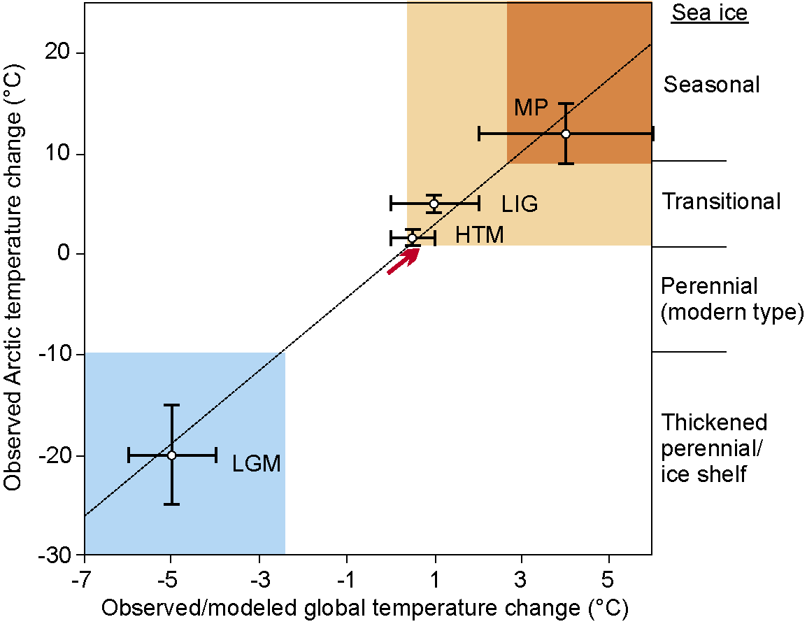
Figure 1: Schematic representation of Arctic sea-ice conditions inferred from paleoclimatic data (e.g. Polyak et al. 2010; Funder et al. 2011; Polyak and Jakobsson 2011). Paleo-temperature anomalies are shown for Last Glacial Maximum (LGM; ~20 ka), Holocene Thermal Maximum (HTM; ~8 ka), Last Interglaciation (LIG; ~130 ka), and middle Pliocene (MP; ~3.5 Ma) (from Miller et al. 2010). Punctured trend line represents the Arctic Amplification. Red arrow shows instrumentally observed temperature change, consistent with observed loss of sea ice approaching the “transitional” state with increasingly large seasonally ice-free areas (see accompanying paper by Serreze and Stroeve).

Due to these limitations one should not expect too accurate predictions of the future course and rate of ice retreat from paleo records; nevertheless, they contain a plethora of information on the state of the Arctic system at different climatic conditions of a much wider range than that of the recent centuries (Fig. 1). Notably, paleo data could shed light on the functioning of the seasonally mostly ice free Arctic and its role in the global climatic ensemble, which is essential for predicting environmental change in the very near future (e.g. Serreze and Barry 2011). One critical set of questions relates to the fate of Arctic biota, from microscopic organisms to polar bears, uniquely adapted to live in or in connection with a perennially ice-covered ocean. Disruption of habitats and life cycle of many Arctic species with shrinking sea ice and increasing temperatures is already underway, along with a northward migration of lower-latitude biota from both the Atlantic and Pacific oceans (Wassmann 2011, and references therein). Striking examples are the penetration of the Pacific diatom Neodenticula seminae via the Arctic into the North Atlantic (Reid et al. 2007) and the distribution of the coccolithophore Emiliania huxleyi from the Atlantic to the northern edge of the Barents Sea (Hegseth and Sundfjord 2008). Stratigraphic data indicate that these migrations likely happen for the first time since the end of the Early Pleistocene (ca. 800 ka) and the Last Interglaciation (ca. 130 ka), respectively.

Investigation of these and other relatively warm, low-ice time intervals of the past few million years, from the current interglaciation (Holocene) to Pliocene, when the Arctic paleogeography was generally similar to modern, has a potential to clarify questions related to the survival of Arctic biota and other impacts of reduced sea ice. This task, however, is complicated by the paucity of paleobiological/biogeochemical proxies in Arctic sediment records because of low marine primary production, overwhelming inputs of terrigenous organic matter, and widespread dissolution of both calcareous and siliceous material, as well as problems with reconstructing sea-ice conditions, which cannot yet be definitively evaluated by any known single proxy. Another complication arises from difficulties with establishing age constraints for Arctic Ocean sediments due to various adverse impacts of the ice cover. Recent achievements in developing sea-ice proxies and improving age controls are encouraging (Polyak and Jakobsson, 2011, and references therein), but much more needs to be done. Promising steps in this direction are underway such as the ESF program Arctic Paleoclimate and its Extremes (APEX) and the newly created PAGES working group on Sea Ice Proxies (SIP), and we can hope for exciting breakthroughs in the near future.

selected references

Full reference list online under: http://pastglobalchanges.org/products/newsletters/ref2012_1.pdf

Miller GH et al. (2010) Quaternary Science Reviews 29: 1779-1790

Polyak L el al. (2010) Quaternary Science Reviews 29: 1757-1778

Polyak L and Jakobsson M (2011) Oceanography 24: 52-64

Serreze MC and Barry RG (2011) Global and Planetary Change 77: 85-96

Wassmann P (2011) Progress in Oceanography 90: 1-17

Solids or liquids suspended in the atmosphere – aerosols – influence Earth’s climate by interacting directly with radiation, by modifying clouds and by perturbing biogeochemical cycles and atmospheric chemistry. Aerosols consist of sulfates, organic carbon, black inorganic carbon, sea spray, mineral dust, ammonia and nitrates, and are emitted either directly or are formed from gaseous precursors. They are released by fossil fuel combustion, biomass burning or by emissions from the land and ocean surfaces. Aerosols reside in the troposphere for less than a day to a few weeks, and up to a few years in the stratosphere (Mahowald et al. 2011).

We monitor aerosols today using ground-based and satellite-borne remote sensing devices, and by in situ sampling on the ground and via aircraft, both at local and global scales (for example, the NASA Global Aerosol Climatology Project). But, despite the large number of observations of aerosols, there are large uncertainties in their distribution in space and time and their characteristics, because of their variability in space, time and composition (Mahowald et al. 2011; Formenti et al. 2011). In addition, aerosol deposition can be studied using passive natural or human-made collectors, such as snow pits or marine sediment traps (Kohfeld and Harrison 2001). Increasingly complex atmospheric transport and chemistry models and Earth-system models complement the set of tools for the study of the aerosol-climate interactions (Stier et al. 2006).

In its fourth assessment report, the Intergovernmental Panel on Climate Change estimated that anthropogenic aerosols had a net cooling effect on climate, partly offsetting the warming from greenhouse gases. But this conclusion is tempered by the large uncertainties involved. Aerosol-climate interactions thus constitute one of the major sources of uncertainty in assessing the global average radiative forcing (RF; Forster et al. 2007), and contribute to the large uncertainty in climate sensitivity (globally averaged surface temperature change at equilibrium) of between 2 and 4.5°C for doubling of CO2 (IPCC 2007).

Aerosols affect the climate in multiple ways. The direct effect – by scattering and absorption of solar and terrestrial radiation – leads to an RF value of -0.50±0.40 Wm-2 compared to the +1.7±0.1 Wm-2 estimated for rising CO2 levels (Forster et al. 2007). Similarly, this interaction of aerosols with radiation also appears to be contributing to the observed “dimming” or reduction in the amount of incoming solar radiation that reaches the surface (e.g. Haywood et al. 2011). Aerosols interact with clouds by modulating albedo (the “cloud albedo” effect), which causes RF of -0.7 (-0.3 to -1.8) Wm-2, and by modifying cloud lifetime (Forster et al. 2007). Aerosols also modify biogeochemical cycles by providing nutrients that limit primary production (e.g. Martin et al. 1990) and by producing climate alterations, which in turn enhance carbon uptake, affecting climate indirectly with an estimated RF of -0.50±0.40 Wm-2 (Mahowald 2011). In addition, deposition of black carbon and dust modify the albedo of snow (Hansen and Nazarenko 2004).

Natural aerosols are a potent source of feedbacks to the climate (Carlsaw et al. 2010). The impact of stratospheric aerosols on climate is seen in the response of the surface cooling to large volcanic events (e.g. Mt. Pinatubo), which can be as large as -0.2°C globally averaged (Robock 2000). Because of the potency of aerosols for climate perturbation, they are also being considered for tools in geoengineering the climate (e.g. Shepherd et al. 2009).

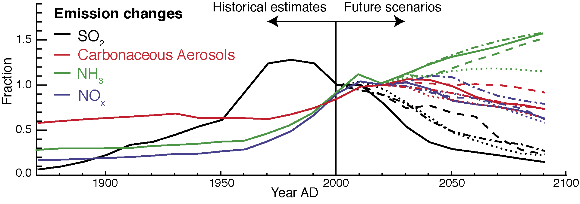
Figure 1: Historical and projected aerosol emissions relative to 2000 AD emissions. Sulfur dioxide forms sulfate aerosols, while about half the ammonia and nitrogen oxides form nitrogen-based aerosols in the atmosphere. Carbonaceous aerosols include both black and organic carbon and the estimated emissions here do not include secondary aerosol formation in the atmosphere. Calculations based on Mahowald (in press).

Humans have significantly increased the amount of aerosol in the atmosphere over the last 130 years. In the future, because of public health concerns as well as efforts to reduce combustion of fossil fuels, it is likely that emissions of anthropogenic aerosols will decrease (Fig. 1). This reduction in aerosols in the future is likely to both increase the rate of warming (Andreae et al. 2005), as well as make reductions in carbon dioxide harder to achieve (Mahowald 2011), because of the complicated and central role of aerosols in modulating climate and biogeochemistry.

selected references

Full reference list online under: http://pastglobalchanges.org/products/newsletters/ref2012_1.pdf

Andreae MO, Jones CD and Cox PM (2005) Nature 435: 1187-1190

Carslaw KS et al. (2010) Atmospheric Chemistry and Physics 10: 1701-1737

Haywood JM et al. (2011) Journal of Geophysical Research 116, doi: 10.1029/2011JD016000

Mahowald N (2011) Science 334, 794-796

Mahowald N et al. (2011) Annual Reviews of Environment and Resources 36: 45-74

Paleoclimate records spanning the past several million years reveal large variability in the deposition of aeolian dust and other natural aerosols. Understanding this variability represents both a challenge and a useful test for Earth system models. The production, transport and deposition of natural aerosols are controlled by numerous physical and biogeochemical processes that are still not well understood. On the other hand, aerosols affect the climate via a number of physical and biogeochemical processes (see the accompanying article by Albani and Mahowald). On short time scales (several years), sulfur aerosols from volcanic eruptions play a significant role in forcing climate. On longer time scales, it is believed that climate-aerosol feedbacks amplify climate changes caused by other factors, such as changes in Earth’s orbital parameters and concentrations of greenhouse gases.

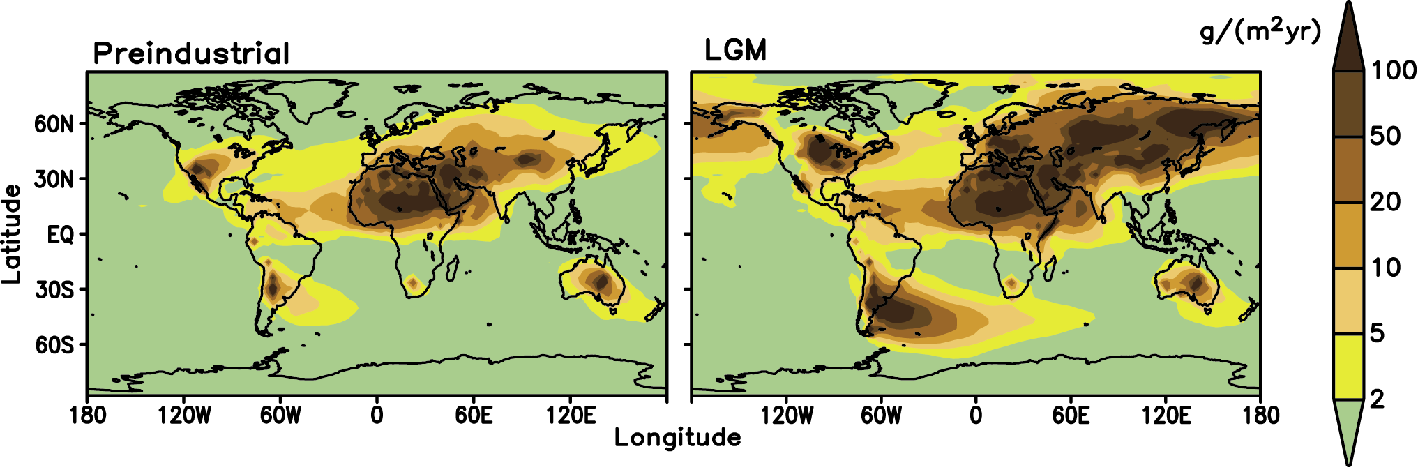
Figure 1: Modeled dust deposition under preindustrial climate conditions (left) and Last Glacial Maximum (right) based on Mahowald et al. (2006).

Variability of the dust cycle is especially significant at glacial-interglacial time scales (Fig. 1). Paleoclimate data and model simulations suggest that during the Last Glacial Maximum (ca. 21,000 years before present) dust deposition in tropics was several times higher than at present and over Antarctica and Greenland the dust deposition rates increased by more than an order of magnitude. Such large increase in atmospheric dustiness cannot be explained without invoking a large increase in dust sources during glacial times (Mahowald et al. 2006). There are a number of processes via which variations in atmospheric dust loading and deposition rates may contribute as amplifiers and modifiers of the orbitally forced glacial cycles. First, an increase in atmospheric dustiness leads to increased reflection of incoming solar radiation and thus contributes to global cooling. This effect can be additionally enhanced by the effect of natural aerosols on cloud albedo (the so-called indirect effect), but partly offset by the additional absorption of outgoing long-wave radiation by dust particles (Takemura et al. 2009). The net simulated climatic effect of dust on climate during glacial times is sensitive to the poorly known optical properties of dust and is therefore model-dependent but typically of a comparable magnitude (1-2 W/m2) to other climatic factors, such as a lowering of the atmospheric CO2 concentration and increased surface albedo due to ice sheet growth. At the same time, enhanced dust deposition over snow and ice leads to a reduction of surface albedo and thus enhances ice melt. This effect may have played a role in both preventing the ice sheets from spreading into lower latitudes (Krinner et al. 2006) and accelerating the retreat of the ice sheets during glacial terminations (Ganopolski et al. 2010).

In addition to the physical effect, enhanced deposition of dust over ocean areas where plankton growth is limited by the availability of iron can enhance biological production and thus lead to the drawdown of atmospheric CO2 (Martin et al. 1990). Recent modeling experiments suggest that the iron fertilization effect in the Southern Ocean alone can explain a significant fraction of glacial CO2 reduction (Brovkin et al. 2007). Further progress in understanding the role of dust and other natural aerosols in climate change therefore requires the incorporation of these processes into the new generation of Earth system models.

selected references

http://pastglobalchanges.org/products/newsletters/ref2012_1.pdf

Brovkin V, Ganopolski A, Archer D and Rahmstorf S (2007) Paleoceanography 22, doi: 10.1029/2006PA001380

Ganopolski A, Calov R and Claussen M (2010) Climate of the Past 6: 229-244

Krinner G, Boucher O and Balkanski Y (2006) Climate Dynamics 27(6): 613-625

Mahowald N et al. (2006) Journal of Geophysical Research 111, doi: 10.1029/2005JD006653

Takemura T et al. (2009) Atmospheric Chemistry and Physics 9: 3061-3073

Historic changes in land use have altered the land surface significantly. For example, since the early 19th century, there has been a substantial increase in the area of cropland in the middle latitudes of the Northern Hemisphere. The pronounced tropical deforestation during the 20th century has paralleled the large-scale development of urban settlements and irrigated agriculture. The land-cover changes have resulted in a number of alterations in the regional and global climate system, primarily by: 1) Changing the surface albedo; 2) Changing the surface evapotranspiration; 3) Modifying winds, heat wave resilience, vulnerability to floods and other such factors in the proximity of human settlements; and 4) Modifying atmospheric CO2 uptake.

Figure 1: Effects of land use and CO2 forcings on temperature change from pre-industrial to present-day in two heavily deforested areas (central North America and central Eurasia) as simulated with seven atmosphere-land models (de Noblet-Ducoudré et al. in press). Most simulations suggest that the propagating land use resulted in significant regional cooling, which approximately counteracted the concurrent CO2-related warming in these regions.

Changes in the albedo and evaporation have likely had a discernible effect on global mean temperatures since the late 19th century, although models show varying results of the net effects on climate (Pitman et al. 2009). Decreased forest cover has generally increased the surface albedo, thereby reducing the net energy available at the surface. This has possibly led to a downward modulation of the global mean warming rate (approximately 0.7°C since instrumental measurements began; IPCC 2007) by 0–0.1°C (de Noblet-Ducoudré et al. in press). Local land-atmosphere feedbacks generate large spatial variability of the land-use effects. In general, land-use-induced temperature changes are relatively small in the tropics, but increase significantly while moving to the equator. In areas with large deforestation (e.g. USA, central Eurasia) the local cooling has likely more than compensated for the global mean warming induced by elevated greenhouse gas concentrations (de Noblet-Ducoudré et al. in press; Fig. 1), although this finding needs to be balanced with the fact that deforestation itself has significantly contributed to the increase in CO2 (Pongratz et al. 2010). Net effects of land use on evaporation are more uncertain than those on albedo. Higher evaporation may be alternatively found over forests or grassland depending on the local conditions (Teuling et al. 2010).

Apart from the direct impacts on the physical climate system, large-scale deforestation has resulted in a significant release of carbon to the atmosphere, adding to the CO2-perturbation caused by fossil fuel burning. On top of the estimated 9.1±0.5 Gt carbon released from fossil resources in 2010, another estimated 0.9±0.7 Gt carbon was released by land-use change (Peters et al. 2011). Through the combination of CO2 and biophysical effects, deforestation is expected to lead to a net climate warming in tropical regions, but possibly to a net cooling in boreal regions (Betts et al. 2007, Bonan 2008). However, human management could also play a role, because areas that are deforested tend to have higher carbon content and less snow cover (Pongratz et al. 2011). Another marked effect of land-use change on climate is an increase in vulnerability to climate extremes, both because of the potential inability of forest areas to dampen temperature extremes during the early heatwave stages, and because of the increased exposure to extreme events like floods.

In the context of the 5th Coupled Model Intercomparison Project (CMIP5), many Global Circulation Model projections have been carried out for a number of future socio-economic scenarios, including land-use change. Early results indicate that the overall magnitude of projected land-use change (that is, the conversion of natural vegetation to cropland) is generally smaller than observed during the 20th century in all future scenarios. The regional differences, however, are pronounced. Sub-Saharan Africa is projected to experience a significant increase in agricultural area in most of the scenarios, even in the low-emission scenario targeted to meet the 2-degree global warming criterion. The local expression of land-use interaction with climate and the large spatial variability of the nature and degree of land-use change calls for an increasing focus on assessing impacts of land-cover change at a regional level.

selected references

Full reference list online under: http://pastglobalchanges.org/products/newsletters/ref2012_1.pdf

Bonan GB (2008) Science 320: 1444

de Noblet-Ducoudré N et al. (in press) Journal of Climate, doi: 10.1175/JCLI-D-11-00338.1

Peters GP et al. (2011) Nature Climate Change 2: 2-4

Pitman AJ et al. (2009) Geophysical Research Letters 36, doi:10.1029/2009GL039076

Pongratz J et al. (2011) Geophysical Research Letters 38, doi: 10.1029/2011GL047848

Teuling AJ et al. (2010) Nature Geoscience 3: 722-727