PAGES Magazine articles
Didier Galop1, T. Houet1, F. Mazier1, G. Leroux2 and D. Rius1
1Laboratory GEODE UMR 5602 CNRS (GEOgraphie De l’Environnement), University of Toulouse, France; didier.galop univ-tlse2.fr
2ECOLAB UMR 5245 CNRS, University of Toulouse, France
Reconstruction of the relationship between pastoral activities and vegetation history in the central Pyrenees demonstrates the importance of grazing pressure in the maintenance of floristic diversity in highland regions that have been abandoned.
In the context of biodiversity management, as encouraged by the European Union Habitats Directives and by the implementation of national strategies, the preservation of traditional agro-pastoral farming activities (in particular extensive grazing), is a major issue acting to maintain or restore open land that is favorable to biodiversity. Here, we present a case from the Pyrenean Mountains, which is considered the most important mountainous massif in southern Europe due to its biodiversity and high levels of endemism. Since the mid 20th century, agricultural activities in these mountains have significantly declined, often accompanied by a change in grazing practices. From a pastoral point of view, the current situation in the Pyrenees is complex. In the Eastern Pyrenees, grazing areas are being abandoned, which is resulting in an expansion of heathland and forest. Conversely, in the Central and Western Pyrenees, an intensification of grazing is observed. This intensification creates problems that are characteristic of overgrazed areas; soil erosion and the fragmentation of animal habitats by fences. European and national policies are attempting to face this situation, where over-grazing and abandonment coexist, through support of conservation organizations, such as the Pyrenees national park, the regional natural parks, natural reserves, and nature charities, which participate in the local implementation of the networking program “Natura 2000” (Magda et al., 2001). The development of a co-management structure, with involvement of local and governmental environmental managers, is encouraged in order to set up strategies reconciling biodiversity conservation with restoration or maintenance of agro-pastoral activities. Pastoral activities are considered essential for maintaining open land, preventing the expansion of invasive species, and forestalling secondary succession of forests following past anthropogenic activities. For the majority of cases, a return to extensive grazing activities is highly recommended. However, this suggestion is often based on present-day observations with a temporal record spanning no more than 10 years (Canals and Sebastià, 2000).
The potential of incorporating historical ecology and paleoecology in conservation biology is now recognized, including their applicability to biodiversity maintenance, conservation evaluation and changing disturbance regimes. Paleo-studies can provide guidelines for environmental managers (Swetnam et al., 1999; Valsecchi et al., 2010). The effects of long-term, human-induced disturbances (i.e., grazing pressure) on ecosystem dynamics and their biodiversity still need to be further investigated.
A Human-Environment Observatory: Insights on future dynamics
The Upper Vicdessos Valley (Ariège, eastern Pyrenees) is representative of a common scenario in the Pyrenean massif where agro-pastoral activities have reached an extremely low level, now characterized only by extensive grazing. Successional processes involving encroachment of open land and overgrowth by trees are now occurring rapidly at all altitudes. Hill slopes have all been subjected to an overwhelming encroachment of fallow land (Betula, Fraxinus, Corylus) whereas altitude zones used for summer grazing are progressively colonized by heathland (principally Juniperus communis, Calluna vulgaris, Cytisus scoparius). After thousands of years of intense agro-silvo-pastoral activities (going back to the late Neolithic period, Galop and Jalut, 1994), a rapid decline in human activities linked to rural depopulation took place during the first half of the 20th century.
The Vicdessos Valley is therefore a particularly interesting case study. Since 2009, a Human-Environment Observatory (http://w3.ohmpyr.univ-tlse2.fr/presentation_ohm_pyr.php) headed by the laboratory GEODE was set up by the Institute of Ecology and Environment of the French National Center for Scientific Research (INEE-CNRS). It aims to monitor past and present evolutions of human-environment interactions in order to anticipate future dynamics and consequently to provide a scientific basis for understanding the functioning of social-ecological systems. This implies a close collaboration with local and governmental planners in charge of management and conservation of landscapes and ecosystems. The observatory is a multidisciplinary consortium bringing together scientists to work on integrated micro-regional research (Pyrenean Valley scale). It involves observations and measures of present dynamics (e.g., meteorological and climatic observations, experimental approaches, monitoring of plant and animal communities) and studies of past human activities over long-term timescales. The latter uses instrumental and documentary data sources, tree demography (dendrology), old maps, agricultural statistics, aerial photographs, and long-term sedimentary proxy data (e.g., sedimentology, biogeochemistry, pollen and charcoal) from lakes and bogs in the valley.
From over-grazing to abandonment: 200 years of grazing activities
 |
|
Figure 1: Trajectories of changes observed since the beginning of the 19th century in the Bassiès Valley based on historical and paleodata. a) Evolution of the Auzat commune population; b) Comparison between the evolution of grazing pressure recorded in agricultural statistics of the Auzat commune and the estimated palynological richness (E(Tn)) inferred from pollen records from the Orry de Théo peat bog; c) Ash content (mineral fraction; LOI 550°C) recorded in the Orry de Théo peat bog; d) Charcoal (>150 µm) accumulation rate reconstructed in the Orry de Théo peat profile; e) Pollen accumulation rates (g cm-2 a-1) of selected taxa recorded in the Orry de Théo peat bog. This reconstruction shows, at a local scale, the change from a scenario of over-grazing to a near-total abandonment of summer pastoral farming activities. In the 1950s, an important period of transition is noted during which grazing pressure can no longer curb the development of heathland species and tree recolonization (dashed gray line). |
 |
|
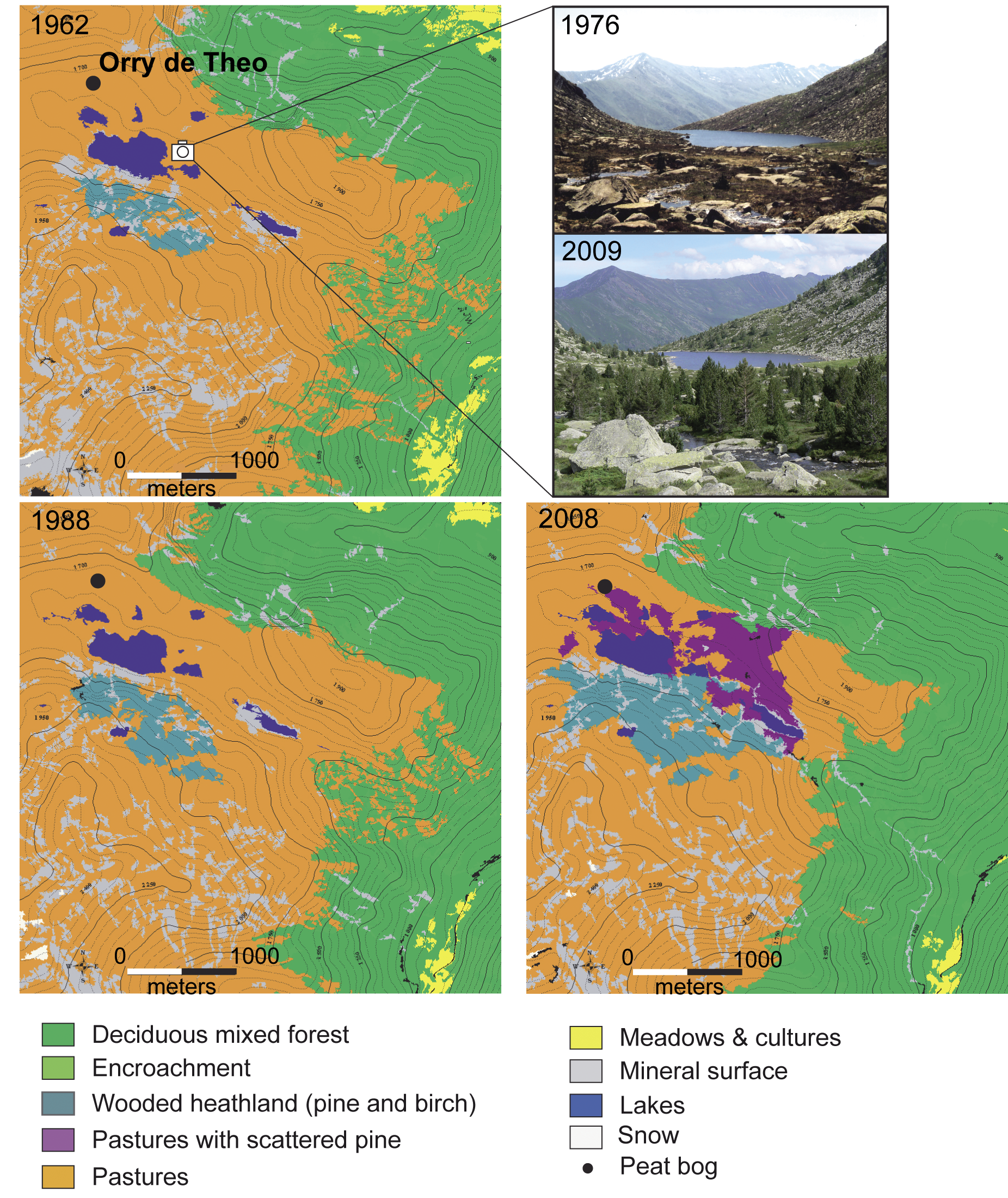
Figure 2: Maps based on aerial photographs (French National Geographic Institute) showing vegetation and land-use changes in the Bassiès Valley between 1962 and 2008. The grazing decline (orange area) is concomitant with increasing forest density, principally dominated by an expansion of Pinus uncinata and birch (aqua and purple areas). This density increase has been particularly rapid during the last 20 years as shown by the repeat photographs taken in the valley’s pastoral zones between 1976 and 2009. |
In the Vicdessos Valley, the hanging valley of Bassiès (altitude between 1400 and 2500 m asl) lies one of the study sites of the observatory. The research focuses on the impact of grazing activities on high-altitude ecosystems. Paleoecological data, including pollen and charcoal (>150 µm) accumulation rates and loss-on-ignition (LOI), have been retrieved from the small peat bog of Orry de Théo. This sequence illustrates the history of vegetation cover, soil erosion and fire in relation to grazing activities over the last 200 years (Fig. 1). Rarefaction analysis was undertaken on pollen data to estimate the variations of palynological richness assumed to reflect the floristic diversity, and vegetation and landscape dynamics over time (Berglund et al., 2008). The comparison of the palynological richness with documentary sources (demographic data and book records of number of cattle in the valley) provides valuable insights on the role of human-induced disturbances such as grazing activities on floristic and landscape diversity. Figure 1 shows a positive association between grazing pressure and floristic richness. This correlation remains high until around the 1920s despite a decrease in sheep numbers, whereas the presence of cattle leads to soil degradation. A threshold is reached in the 1950s: the decline of flocks associated with a modification of pastoral practices leads to under-grazing and limits the soil erosion. At the same time, the overgrowing of Juniper and Calluna heathlands and the expansion of trees (Pinus and Betula), no longer controlled by browsing, are favored. Fire signatures recorded between 1950 and 1970 may indicate the use of fire by the shepherds to restore and clear their pastures. From the beginning of the 1980s, a significant reduction in the number of farmers in the valley has progressively led to a near-total disappearance of grazing activity. In these previously grazed areas, an inevitable and probably irreversible (except through expensive restoration actions) return to forest has led to a decline in floristic diversity. Landscape dynamics are illustrated by reconstructions based on aerial photographs taken between 1962 and 2008 as well as repeat photographs showing the progression of pine-dominated forest between 1976 and 2009 (Fig. 2). The correspondence between paleoecological data and documentary sources confirms the complementarity of the approaches.
The local case study of the Bassiès Valley gives information on diversity baselines, thresholds, and the resilience of mountainous ecosystems to anthropogenic disturbances. This study is also rich in lessons on the loss of floristic diversity related to the variability or the decline in grazing activities and to pine-dominated secondary succession in a context of under-grazing. This kind of integration of data is already being used by managers to affirm the necessity or futility of restoration actions, and especially to avoid thresholds and to reverse the trajectories of key processes.
references
For full references please consult: pastglobalchanges.org/products/newsletters/ref2011_2.pdf
Thomas Foster
University of West Georgia, Carrollton, USA; tfosterwestga.edu
This article discusses how long-term regional data from historic documents, palynology and archeology are combined to inform decisions about biodiversity management in the southeastern United States.
The United States proactively manages federally owned lands with an objective to mitigate/limit the impacts of land-use activities on the long-term stability of the environment. For example, the United States Department of Defense (DoD) manages around 25 million acres of national military land. Impacts of military land use can include soil erosion, loss of endangered species, and degradation of habitats (Goran et al., 2002). Management involves planning and assessment that takes into consideration the types of environment to be managed and how they have changed over time, in order to maintain lands for training and operations. Fort Benning, founded in 1920, is a military base in Georgia and Alabama in the southeastern United States. It covers an area of 1052 km2 and is situated near the fall line of the Coastal Plain where soils consist of clay beds and sandy alluvial deposits (Fenneman, 1938). The pre-European (before ca. AD 1825) forest was primarily a pine-blackjack oak forest (Black et al., 2002). This article summarizes some recent research on long-term environmental changes and how it is being used to manage current ecological problems.
Ecological Problems
At Fort Benning, management challenges include protection of federally endangered Red Cockaded Woodpecker (Picoides borealis) and habitats important to rare species, such as the Gopher Tortoise (Gopherus polyphemus) and relict Trillium (Trillium reliquum) (Addington, 2004), as well as combating erosion (Fehmi et al., 2004). Proscribed forest fires have to be scheduled so as to maximize ideal training environments (e.g., reduced undergrowth) and preserve a forest composition that is conducive to species diversity and protects endangered species. Environmental managers at Fort Benning not only need to understand the long-term dynamics of the landscape but must also have the management tools for planning.
Therefore, as highlighted in a series of recent publications (Dale et al., 2002; Dale et al., 2004; Dale and Polasky, 2007; Foster, 2007; Foster et al., 2004; Foster and Cohen, 2007; Foster et al., 2010; Goran et al., 2002; Olsen et al., 2007), the DoD has funded research at Fort Benning focused on identifying long-term ecological metrics, human population settlement, and human activities that may have altered the environment.
Data Sources
 |
|
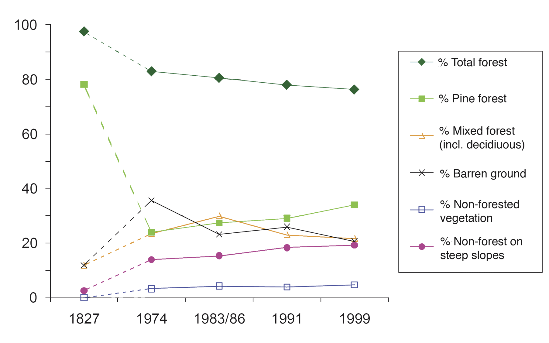
Figure 1: Graph showing the relative abundance of forest cover at Fort Benning, Georgia from 1827-1999 (adapted from Olsen et al., 2007). Data were collected from historic documents and satellite imagery. |
Environmental management at Fort Benning has included the use of archeology, historic documents, historic and modern satellite images, and pollen from sediment cores. For example, historical “witness tree” records reveal pre-European settlement forest composition. Witness trees are boundary markers recorded on land survey maps that were created when lands were acquired by the state and federal government in the late 18th to early 19th century in Georgia and Alabama. The corner trees and four "witness trees" were recorded at the corners of each survey lot (approximately 82 ha), and the species of the trees were noted on maps and field notes. These data provide a record of the forest composition at the time that the Native Americans were removed by state and federal agencies in the early 19th century and represent the pre-European forests and the forests under Native American management. These data were synthesized into a GIS and compared to historical satellite images (1974-1999; Fig. 1). Knowledge of human settlement and its intensity was revealed by systematic sampling of the military base with archeological investigation. The entire base was examined for human activity at 5 to 30 m intervals. The remains of human activity were analyzed for behavior type, intensity, population density, and economic activity. Lastly, long-term forest composition change was provided by analyzing pollen sequences from peat cores. Cores were dated with 137Cs/210Pb and 14C (Foster and Cohen, 2007).
Findings
As revealed through archeological investigations, Native Americans had lived in the Fort Benning region for at least 10,000 years though their management of the forest had changed dramatically in the last 1000 years (Foster, 2007; Kane and Keeton, 2000). European settlement and military activities within the last 100-200 years further affected the modern environment. Comparisons of the Native American managed forest to satellite imagery during the 20th century indicates that the land cover at Fort Benning has changed significantly (Olsen et al., 2007). The prevailing trend is a decrease in pine and increase in deciduous forest (Fig. 1). Pine forest cover decreased from nearly 80% to below 40% from 1827 to 1999. The increase in deciduous forest is mostly associated with riparian areas, as the riparian areas became larger (Olsen et al., 2007). Forest cover was cut down soon after this area was settled by United States citizens, which resulted in increased soil erosion and habitat degradation (Foster and Cohen, 2007).
 |
|
Figure 2: A) Pollen abundance from the Hite Bowl site, Fort Benning, Georgia (adapted from Foster and Cohen 2007). B) Same as A) for the Beaver Dam site. These two plots illustrate the localized effect of human activity on vegetation cover. |
Analysis of pollen and charcoal from sediment cores revealed that change in forest composition was localized and affected by human activity. Figure 2 shows the significant changes in pollen composition since Native Americans were removed from the region around 1830. Pinus and Nyssa have increased in some localized areas whereas Sphagnum has decreased. The Native Americans had localized effects on pine and some hardwood species.
Lessons for management
Archeological data, in combination with analysis of pollen, charcoal and fungi from sediment cores (Foster and Cohen, 2007), indicate that the long term effects of human activity are highly localized. Sediment core data indicates that in areas where Native American settlement was dense, pine forest has increased dramatically since European and military settlement (Foster and Cohen, 2007). While in the areas where native people were less densely settled, pine forest has remained approximately the same (Fig. 2; Foster and Cohen, 2007).
Overall, the management plan at Fort Benning has prescribed intensive land use in some areas while preserving others. Based on comparisons of forest composition inside the base to that outside the base, this plan has increased the habitat for endangered species, such as the Red-Cockaded Woodpecker (Picoides borealis), to a level that is higher than the regions outside of the military boundary (Olsen et al., 2007). Long-term data have also revealed the localized effects of management policies and are being used to design better policies that are sensitive to the range of biological diversity at Fort Benning.
The combination of long-term data on human settlement and economic activity combined with long-term ecological data reveal that the modern management of forest ecosystems is complicated and regionally variable. Though these data were recovered using diverse methods and varying units of investigation, they can be combined for regional analysis of long-term environmental change. Management decisions that cross ecological regions will likely include variable human activities and ecological conditions. In the case of Fort Benning, modern management has increased pine density beyond that created by pre-European settlement in one region and decreased pine density in another region beyond that of the pre-European forests. An understanding of this process can only be gained through regional analysis of long-term environmental data combined with anthropological understanding of human activities. These data permit modern forest managers to understand the long-term effects of anthropogenic change and the interaction of those changes with the forest ecosystem. Such a long-term perspective is leading to better informed management practices.
data
Data referenced in this article are available at http://semp.cecer.army.mil
references
For full references please consult: http://pastglobalchanges.org/products/newsletters/ref2011_2.pdf
Colleen E. McLean1, D.T. Long2 and B. Pijanowski3
1Department of Geological and Environmental Sciences, Youngstown State University, USA; cemcleanysu.edu
2Department of Geological Sciences, Michigan State University, USA
3Department of Forestry and Natural Resources, Purdue University, West Lafayette, USA
Sediment geochemistry and diatom biostratigraphy can be used to identify stressor-response relationships in aquatic ecosystems for improved regional management strategies.
Aquatic ecosystems in the Great Lakes region of North America have been significantly altered since Euro-American settlement in the late 1700s. Human activities contributing to environmental degradation initially included population increase, land use change, and dramatic industrialization (Alexander, 2006). An understanding of the state of modern aquatic ecosystems can be gleaned from reconstructing the environmental history of the region. Integrating historical records with high-resolution paleolimnological data is an effective way to capture stressor-response relationships and evaluate human influence. These relationships facilitate an understanding of comprehensive aquatic ecosystem response, and are useful for developing predictive tools for future anthropogenic influences. Having such tools is critical for developing sustainable management strategies, and can be used directly by decision makers at the regional scale.
Impacts in the Laurentian Great Lakes Region
A sediment core from Muskegon Lake, Michigan, USA, was analyzed for multiple proxies to assess the system’s response and recovery to human activity, with particular attention to ecosystem recovery since the introduction of environmental legislation in the United States (e.g., Clean Air and Clean Water Acts). Muskegon Lake is a 16.91 km2 inland water body located in the Laurentian Great Lakes region (86°18’ W, 43°14’N) (Parsons et al., 2004). Its mean depth is 7 m with a maximum depth of 23 m. Muskegon Lake itself is the end point of a drowned river mouth system that connects the Muskegon River Watershed to the coastal zone of Lake Michigan through a navigation channel (Steinman et al., 2008). This proximity to the Great Lakes and general ecological setting make it an important fishery, though invasive species, habitat loss and degradation continue to be factors of concern (Lake Michigan Lakewide Management Plan, 2004).
 |
|
Figure 1: Trends of land use change since 1900 (Ray and Pijanowski, 2010) for the Muskegon River Watershed (location green on map inset), population data for Muskegon county since 1860 (US Census) and regional scale human impacts since Euro-American settlement. WWTP = Wastewater Treatment Plant. |
Muskegon Lake has a history of intense anthropogenic activity since the early 1800s (summarized in Fig. 1). During the lumber peak in the 1880s, the city of Muskegon had more than 47 sawmills. Following the depletion of lumber resources, Muskegon developed an industrial base, with oil and chemical industries being prominent (Alexander, 2006). In the mid-1900s, foundries, metal finishing plants, a paper mill and petrochemical storage facilities were built on the shore of Muskegon Lake (Steinman et al., 2008). Expansion of heavy industry and shipping in 1960s and 1970s contributed to over 100 000 m3/day of wastewater discharged from industrial and municipal sources into the lake until a tertiary Waste Water Treatment Plant (WWTP) was installed in 1973 (Freedman et al., 1979; Steinman et al., 2008). Currently, there are eight abandoned hazardous waste sites (USEPA Superfund sites) in the region and fish consumption advisories have been issued due to significant levels of PCB (Polychlorinated biphenyls) and mercury.
Environmental response to regional impacts
 |
|
Figure 2: A) Profiles of select anthropogenic elements with concentrations normalized to highest concentration of each element, B) Normalized sediment phosphorus (P) profile (as a measure of water quality) with measured concentrations of water column soluble reactive P and water column total P from 1972 and 2005 (Freedman et al., 1979; Steinman et al., 2008), and C) Relative abundances of select fossil diatoms indicative of water quality changes. |
Analyses of geochemical data from the sediment core showed suites of elements that corresponded to the source of the sediment, including terrestrial in wash, primary productivity, redox sensitive and anthropogenic related material (Long et al., 2010; Yohn et al., 2002). Elements influenced by terrestrial processes (e.g., Al, K, Ti and Mg) reflected drowned river mouth conditions of Muskegon Lake, and recorded deforestation-induced erosion in the late 1800s. Productivity related elements (e.g., P and Ca) indicated changes with nutrient inputs to the lake (presumably related land use change). Redox sensitive elements (e.g., Fe and Mn) were important for interpreting the redox state of the system. Elements associated with anthropogenic activity (e.g., Cr, Pb and Sn) had similar profiles, which closely track the history of human activity (see Fig. 2A), though concentration peaks for individual elements varied by specific industrial activity. For example, driven in part by policy mandates (e.g., discontinued use of leaded gasoline) Pb decreased to ~60 ppm in modern sediment from a peak of ~325 ppm, reflecting significant recovery from peak concentrations of anthropogenic elements. However, the Pb values did not return to the pre-disturbance Pb concentration of ~11 ppm. The geochemical reference condition was evaluated using sediment concentration profiles of the anthropogenic proxy group, which best indicates the pre-Euro/American settlement conditions. Results show that modern concentrations of anthropogenic elements have not decreased to the historical geochemical reference condition (e.g., Pb).
Biological change in Muskegon Lake, inferred from fossil diatoms, suggests that the pre-settlement community structure is markedly different from that of modern assemblages. Figure 2 includes specific diatom biostratigraphic changes that correspond to the timeline of various human stressors, including water chemistry changes resulting from agricultural development, industrialization and urbanization of the watershed. For example, taxa indicating high nutrient conditions (e.g., Stephanodiscus spp.) have peak abundances dated between 1930s and 1970s when nutrient inputs were increasing due to agriculture and urbanization. Moreover, productivity regimes in the lake, reconstructed from diatom habitat structure, identified a significant shift from planktonic- to benthic-dominated productivity in the top 25 cm of the core; this shift is dated to after the installation of the WWTP in 1973. Much of the water quality improvements in the past 30 years, reported by Freedman et al. (1979) and Steinman et al. (2008), and also noted in Figure 2, are presumably attributed to the WWTP installation. Decreases in lake-wide averages of total phosphorus and soluble reactive phosphorus at the water surface range from 68 to 27 μg/L and from 20 to 5 μg/L, respectively from 1972 to 2005. In addition, average chlorophyll-a concentrations have declined by 19 μg/L over this period, while Secchi disk depths (a measure for water transparency) have increased from 1.5 to 2.2 m (Freedman et al., 1979; Steinman et al., 2008). This partial recovery corresponds to the shift in dominant habitat of primary productivity, as the relative abundance of planktonic dominated taxa at the bottom of the core (i.e., in pre-settlement times) is between 56 and 77%, peaks at 88% in 24 cm depth (dated to 1970 at the peak of cultural eutrophication), and then quickly decreases to 26-37% in the top 8 cm of the core. The productivity shift in the top 8 cm (benthic taxa become 54-64% dominant) may also be influenced by the invasion of Dreissena polymorpha (zebra mussel).
This study identified causal agents at the regional scale directly linked to human activities such as deforestation, agriculture, industry and urbanization with an integration of geochemical and biological data inferred from fossil diatoms. Overall, the state of the lake system has dramatically improved as the result of environmental management efforts, and this study can be used as an indicator for the response of the larger Lake Michigan that it feeds into (Wolin and Stoermer, 2005). However, recent proxy trends (e.g., sediment P) do not indicate that the system has stabilized, suggesting that modern stressors such as climate variability (Long et al., 2010; Magnuson et al., 1997), invasive species (Lougheed and Stevenson 2004; Steinman et al., 2008) and further land use alterations (Ray and Pijanowski 2010; Pijanowski et al., 2007; Tang et al., 2005) whose influence remain uncertain, are likely to influence system recovery.
Recovery challenges and recommendations
Efforts to manage the watershed have reduced the loading of metals and nutrients, improving the ecological health of Muskegon Lake as evidenced by geochemistry and diatom biostratigraphy. The current geochemical conditions demonstrate significant recovery from high concentrations of anthropogenic elements and the fossil diatom record from this core suggests that efforts to reduce nutrient loading have been successful. Despite improvements, these data indicate that the system is still changing in response to human impacts at the regional watershed scale, suggesting that management strategies also need to target non-point source inputs. As such, it is recommended that modern remediation targets consider the legacy and overprint of multiple stressors, as well as be aware of emerging stressors that could further alter ecological dynamics in the larger Great Lakes Region.
acknowledgements
We thank the Great Lakes Fisheries Trust for funding this research, and the Aqueous and Environmental Geochemistry Laboratory at MSU for providing financial and technical support. Glen Schmitt and the Michigan Department of Environmental Quality are recognized for help in the field. Special thanks to Dr. Nadja Ognjanova-Rumenova for diatom taxonomical processing and identification.
references
Freedman, P., Canale, R. and Auer, M., 1979: The impact of wastewater diversion spray irrigation on water quality in Muskegon County lakes, U.S. Environmental Protection Agency, Washington, D.C. EPA 905/9-79-006-A
For full references please consult: http://pastglobalchanges.org/products/newsletters/ref2011_2.pdf
Lucí Hidalgo Nunes
Department of Geography, State University of Campinas, Brazil; luciige.unicamp.br
The growing severity of floods and landslides in the state of São Paulo, Brazil, is related to rapid environmental changes, such as urbanization, deforestation and settlement in hazardous areas, rather than to natural events, and unless more sustainable land-use practices are adopted the impact of these (un)natural disasters might become more severe.
The Problem
The Emergency Events Database (EM-DAT, www.emdat.be/), an international database of disasters maintained by the Centre for Research on the Epidemiology of Disasters (CRED), states that during the period from 1948 to 2010 Brazil was hit by 146 disasters related to precipitation (storms, floods and mass movements) that caused 8627 deaths and affected nearly 3 million people. Approximately 75% of these calamitous episodes have occurred in the last three decades (1980 to 2010) (EM-DAT, 2010). These figures are probably underestimated (Marcelino et al., 2006; Nunes, 2009) but are consistent with other studies that have demonstrated an upward trend in the severity of disasters triggered by precipitation. It has drawn attention to the question of how strongly this dramatic trend is connected to societal changes, with an ever-growing vulnerability to weather and climate episodes (Kunkel et al., 1999; Changnon et al., 2000; Kesavan and Swaminathan, 2006; Araki and Nunes, 2008).
During the second half of the 20th century, urban population increased steadily in Brazil and according to the census of 2010 (IBGE, www.censo2010.ibge.gov.br/), 84.3% of Brazilians live in urban centers. The unplanned growth of cities has led to an increasing inability to house this growing population and to provide adequate infrastructure. Poor regulation has led to inappropriate land use transformation in hazard prone areas, higher pressure on natural resources, lack of appropriate waste treatment and sanitation, violence, and other environmental and societal problems. Rapid urban expansion has the potential to adversely affect ecological dynamics, biodiversity and local climate, as well as patterns of local energy and water consumption.
Land use pattern and natural disasters in the state of São Paulo
The impacts of extreme precipitation events are even more acute in the state of São Paulo, where 21.6% of the Brazilian population is concentrated (95.9% in urban centers) and which contributes 33.1% of the national GDP. Three recent assessments of the historical interactions between climate and social change are providing insight into the controls on landslides and flood:
 |
|
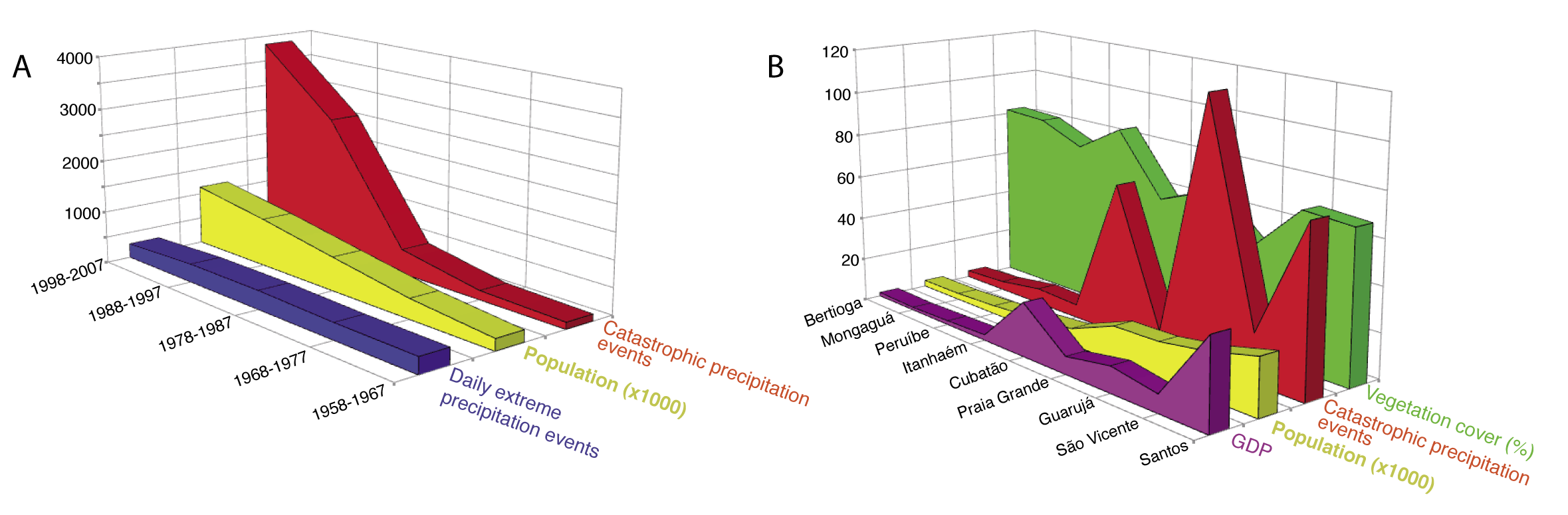
Figure 1: A) Number of catastrophic events caused by precipitation (red) compared with population (yellow) and daily extreme precipitation episodes (blue) in Campinas, Brazil, for 5 decades (1958-1967 to 1998-2007). B) Comparison between Gross Domestic Product (GDP, purple, 2009), population (yellow, 2010), percentage of remaining vegetation (green, 2010) and survey (partially completed) of catastrophic events triggered by precipitation (red) from 1928 to 2009, for 9 municipalities of the Metropolitan Region of Baixada São Paulo, Brazil. Higher number of catastrophic events is related to higher deforestation, and lower GDP to lower rates of deforestation. |
1) Evaluating the consequences of extreme precipitation events between 1958 and 2007 in Campinas (1,080,999 inhabitants, census of 2010), Castellano (2010) observed a significant increase in the number of the impacts (e.g., damages to buildings and trees, power cut and traffic chaos) recorded from 129 impacts in the first decade to 3,837 in the last. During the same period, the population increased by 500%, but no changes in the frequency of extreme precipitation events were recorded (Fig. 1A).
2) The urbanization of Bauru (344,039 inhabitants, 2010) led to decreased soil infiltration with increased runoff released into the natural drainage network, further leading to gullies and more frequent floods. Comparing daily precipitation events above 10 mm/day and erosion and floods from 1967 to 1999, Almeida Filho and Coiado (2001) noticed that the rainfall pattern did not change significantly during the whole period. However, 66% of the episodes occurred between 1984 and 1999, the period of urban population expansion that was not accompanied by urban planning or adequate engineering.
3) The eastern portion of the state, a mountainous region with steep hills at the base of the coastal Serra do Mar Range, is particularly sensitive to natural disasters, with more than 16,000 people living in areas at risk of landslides, mudslides and floods. Some sectors register very intense precipitation episodes. In Cubatão (108,309 inhabitants, 2010), an industrial complex located in a valley surrounded by the unstable hill slopes of Serra do Mar, summer precipitation intensities reached 1021 mm in nine days (February 1929) and 712 mm in two days, (February 1934), as verified by Nunes (2008). In the past few decades Guarujá municipality, an upmarket resort area (290,607 inhabitants, 2010), has experienced an increase in tourism and related activities. This has attracted an influx of workers who largely occupy unstable slopes. As a result, the city has both the highest deforestation rate and highest number of catastrophes triggered by precipitation (floods and landslides) amongst the nine municipalities that are part of the Metropolitan Region of Baixada Santista (MRBS). For the entire area, the correlation between these two variables is -0.85, significant at 95%. Furthermore, the lowest deforestation rates are found in municipalities that also have the lowest GDP, suggesting that the economic development of the region is based on unsustainable practices (Fig. 1B). It is worth emphasizing that this pattern of occupation, with houses perched on steep slopes and next to rivers, is similar to the alpine district of Rio de Janeiro state, where the heavy rains of January 2011 have caused floods, landslides and mudslides resulting in hundreds of deaths and missing persons as well as major economic losses.
 |
|
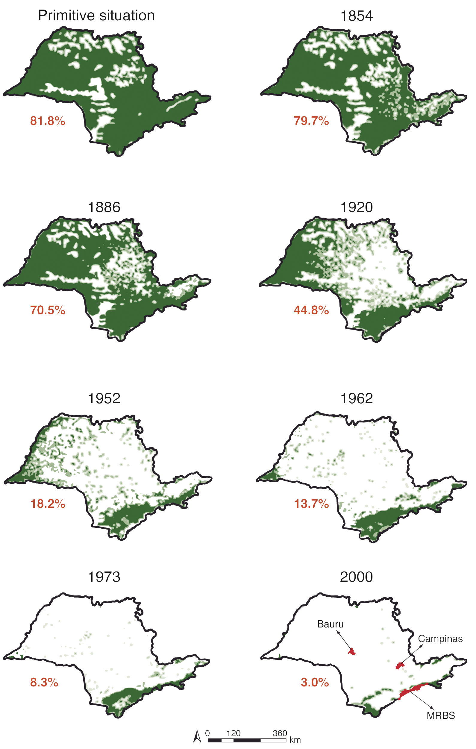
Figure 2: Deforestation of the Atlantic Rainforest in the state of São Paulo from 1854 to 2000. Red numbers indicate the estimation of % forest cover for each period (from Victor, 1975). Red shaded areas indicate location of study areas discussed in the text. MRBS = Metropolitan Region of Baixada Santista. |
Historical information is also being used to highlight the rapid deforestation of the Atlantic Rainforest in recent decades, which is crucial to understanding the recent trends in environmental degradation in São Paulo state. An attempt to reconstruct the forest cover of the state was done by Victor (1975) and Victor et al. (2005) based on reports of pioneers and naturalists, the rise and mobility of population, agriculture expansion and more recently on aerial photo interpretation. It shows that the forest cover of the state was drastically reduced (Fig. 2) by the spread of agriculture and industrialization. The amount of forest cover remaining today corresponds to 2, 8 and 55% of the original area in Campinas, Bauru and Cubatão, respectively.
Future Directions
From the perspectives of both local sustainable development and global change, São Paulo is a “hot spot”. There is a great need to break the cycle of destruction and reconstruction linked to catastrophic events. Knowledge of the extent of historical environmental degradation through depletion of resources, such as has occurred in the Atlantic Forest, and a comprehensive evaluation of the frequency and magnitude of floods and landslides are essential to understanding the evolution of natural disasters. Further studies that take into account the characteristics of the river channel network, the sediment yield from these catchments, the landslide scars, and the weathering and soil development must encompass at least decadal timescales in order to provide rates and nature of changes that take place over planning timescales. The evaluation of current economic development strategies, including policies, guidelines and laws, are vitally important to develop strategies that can lead the entire region towards a more sustainable development trajectory. Planning must be constrained by rules that are defined and rooted in long-term and regional to inter-regional analyses of the optimum and sustainable uses of space.
acknowledgements
I thank Daniel Henrique Candido, PhD student at UNICAMP for the improvement of the figures, and MsD. Ciro Koiti Matsukuma and Valdir de Cicco, Instituto Florestal, for providing the information on deforestation. I also thank Dr. Francisco Sergio Bernardes Ladeira, UNICAMP and Professor John Dearing, University of Southampton, for valuable suggestions.
references
Almeida Filho, G.S. and Coiado, E.M., 2001: Processos erosivos lineares associados a eventos pluviosos na área urbana do município de Bauru, SP.
Araki, R. and Nunes, L.H., 2008: Vulnerability associated with precipitation and anthropogenic factors in Guarujá City (São Paulo, Brazil) from 1965 to 2001, Terrae - Geoscience, Geography, Environment 3(1): 40-45
Castellano, M.S., 2010: Inundações em Campinas (SP) entre 1958 e 2007: tendências socioespaciais e as ações do poder público, Master Dissertation, IG-UNICAMP, (English Abstract)
Victor, M.A. de M., Cavalli, A.C., Guillaumon, J.R. and Serra Filho, R., 2005: Cem anos de devastação: revisitada 30 anos depois, Available at http://antoniocavalli.com/cem%20anos%20de%20devasta%C3%A7%C3%A3o.pdf (English translation)
For full references please consult: http://pastglobalchanges.org/products/newsletters/ref2011_2.pdf
Michael Reid1 and Peter Gell2
1University of New England, Australia; mreid24une.edu.au
2University of Ballarat, Australia
Paleoecological records from billabongs (floodplain lakes) in southern Australia can be used to develop ecosystem response models that describe how the underlying hydrology and geomorphology of these aquatic ecosystems control their resilience to anthropogenic stressors.
Water demands
Lowland floodplain rivers are “hotspots” of biodiversity and productivity. The ecological importance of these environments is particularly substantial in Australian semi-arid and arid environments because of the moisture subsidy they provide to riverine ecosystems (Ogden et al., 2007). In Australia’s dry climate, these environments have also become extremely important for agriculture, which in turn has led to deterioration in ecosystem function and reduced biodiversity. Competing demands for water by ecological and economic systems has led to an apparently intractable debate over how best to allocate water to support sustainable agriculture and ecosystems. The recent debate over the water allocation prescriptions within the Murray Darling Basin Plan (MDBA, 2010) reveal that the changing condition of floodplain wetlands (billabongs) across the region is not well understood. In order to meet this challenge it is vital that water is used efficiently for both agriculture and to support riverine ecosystems. The second half of this equation presents an immense challenge to scientists and managers because our understanding of riverine ecosystem function is limited by a lack of robust data on benchmark conditions, ecosystem variability, and the drivers and trajectories of change.
Ecosystem histories and complexity
Data and information needed to reconstruct ecosystem histories can be provided through paleoecological studies of wetlands. Furthermore, for a basin-wide appreciation, a regional integration of paleoecological studies can reveal the extent and timing of changes to provide broad insights into the ecological cost of the diversion of river flows to support irrigated agriculture.
While factors, such as invasive species and land use, can influence ecosystem structure and function (Roberts et al., 1995; Robertson and Rowling, 2000), floodplain aquatic ecosystems are principally driven by hydrology (Walker, 1985; Bunn et al., 2006). Thus, hydrological changes experienced by billabongs are likely to have a substantial influence on their ecology. However, while the hydrology of a river as a whole is primarily driven by extrinsic factors, the hydrology of individual billabongs is also strongly influenced by intrinsic factors, such as local adjustments in channel morphology, the deposition of sediments in secondary channels linking billabongs to the main channel, and the infilling of the billabongs themselves. Thus individual billabongs may reflect any number of environmental changes operating across a range of spatial and temporal scales. The distinction between local and regional drivers of change can therefore only be revealed by the integration of a suite of studies over a range of hydrological contexts.
Understanding links between stressors and billabong responses is complicated by the fact that billabongs are ecosystems and therefore have system properties such as non-linear and threshold responses to drivers and system resilience. Clearly, billabongs are not passive receptacles that receive sediments and biological remains that reflect linear relationships to broad-scale environmental drivers. Instead, spatial and temporal variability in depositional processes should be anticipated and simple “dose-response”, linear relationships between billabong ecosystems and environmental drivers cannot be assumed. Given this variability and complexity, our capacity to understand the nature, degree, and magnitude of ecological change in lowland river systems is greatly enhanced by robust study designs that incorporate replication of sampling units and a framework for interpreting sediment records that reflects system behavior.
Billabong typologies
 |
|
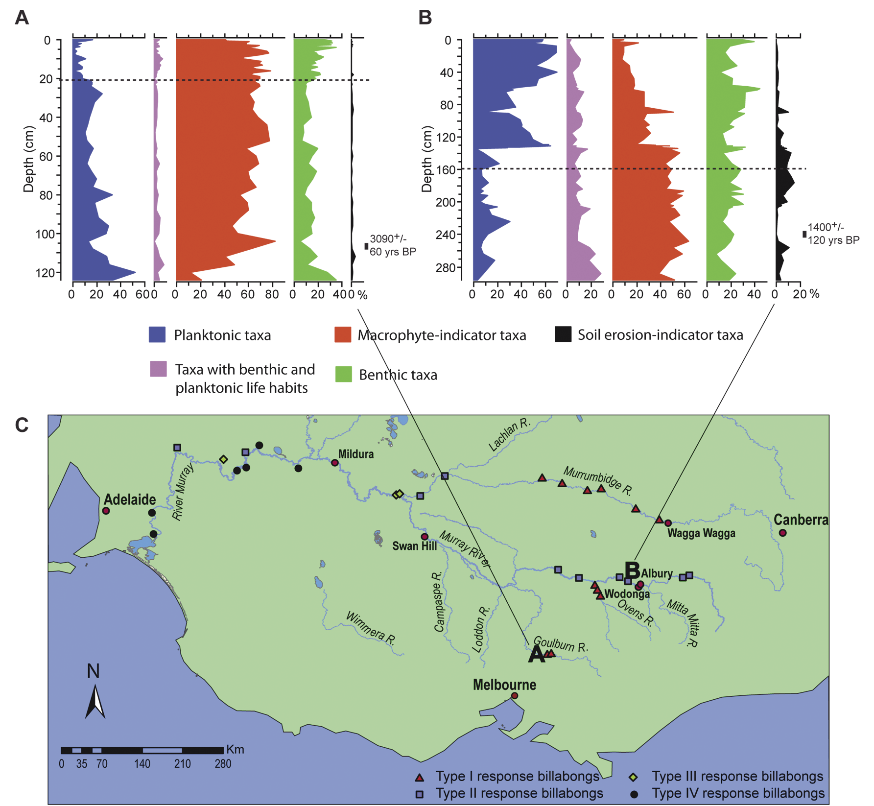
Figure 1: Examples of Type I and Type II responses in billabongs: A) Persistence of macrophyte indicator diatoms (red curve) in a Type I billabong (Callemondah 1 Billabong on the Goulburn River; Reid, 2002) after settlement reflects retention of macrophyte cover, B) Diatom shifts to planktonic dominance (blue curve) in a Type II billabong (Hogan’s Billabong on the Murray River; Reid et al., 2007) after European settlement. Dotted lines indicate onset of post-European settlement sediment deposition in each billabong based on appearance of exotic pollen and physical sediment character, C) Locations of billabongs subject to paleoecological study in the Murray Darling southern basin. Symbols indicate the response type inferred from the paleorecords. |
The utility and value of this approach was demonstrated in early paleoecological research on billabongs in the southern Murray-Darling Basin systems (Ogden, 2000; Reid, 2002, 2008; Reid et al., 2007). Here, large, deep billabongs underwent apparently rapid transitions in state from macrophyte to phytoplankton-dominance at the time of European settlement, while smaller and shallower billabongs maintained substantial submerged macrophyte communities (Fig. 1). The switch from macrophyte- to phytoplankton-dominance was clearly the most significant ecosystem change in those habitats for centuries, and even millennia, and was attributed to reduced photic depth as a result of abiotic turbidity caused by the influx of eroded soils in the region in the mid 1800s. This interpretation is supported by numerous geomorphological studies, which have demonstrated that this period of early settlement was one of intense sheet and gully erosion in south east Australia, driven by the clearing of native vegetation and the introduction of ungulate grazers (Prosser et al., 2001). The patterns observed in these studies highlight the critical importance of photic depth as a driver of ecosystem structure in Australian shallow lakes, a feature demonstrated elsewhere (Scheffer and Carpenter, 2003). A critical aspect of the findings in the southern Murray-Darling Basin was the importance of the underlying morphometry in controlling the system’s resilience to reduced photic depth.
This simple two-response type framework does not appear to apply to billabongs further downstream in the Murray-Darling System. Numerous studies of billabongs and floodplain wetlands on the Murray below the confluence with the Goulburn River have been carried out, and the majority of the records derived from these studies do not conform to one of the types described above (Gell et al., 2005, 2007; Fluin et al., 2010).
 |
|
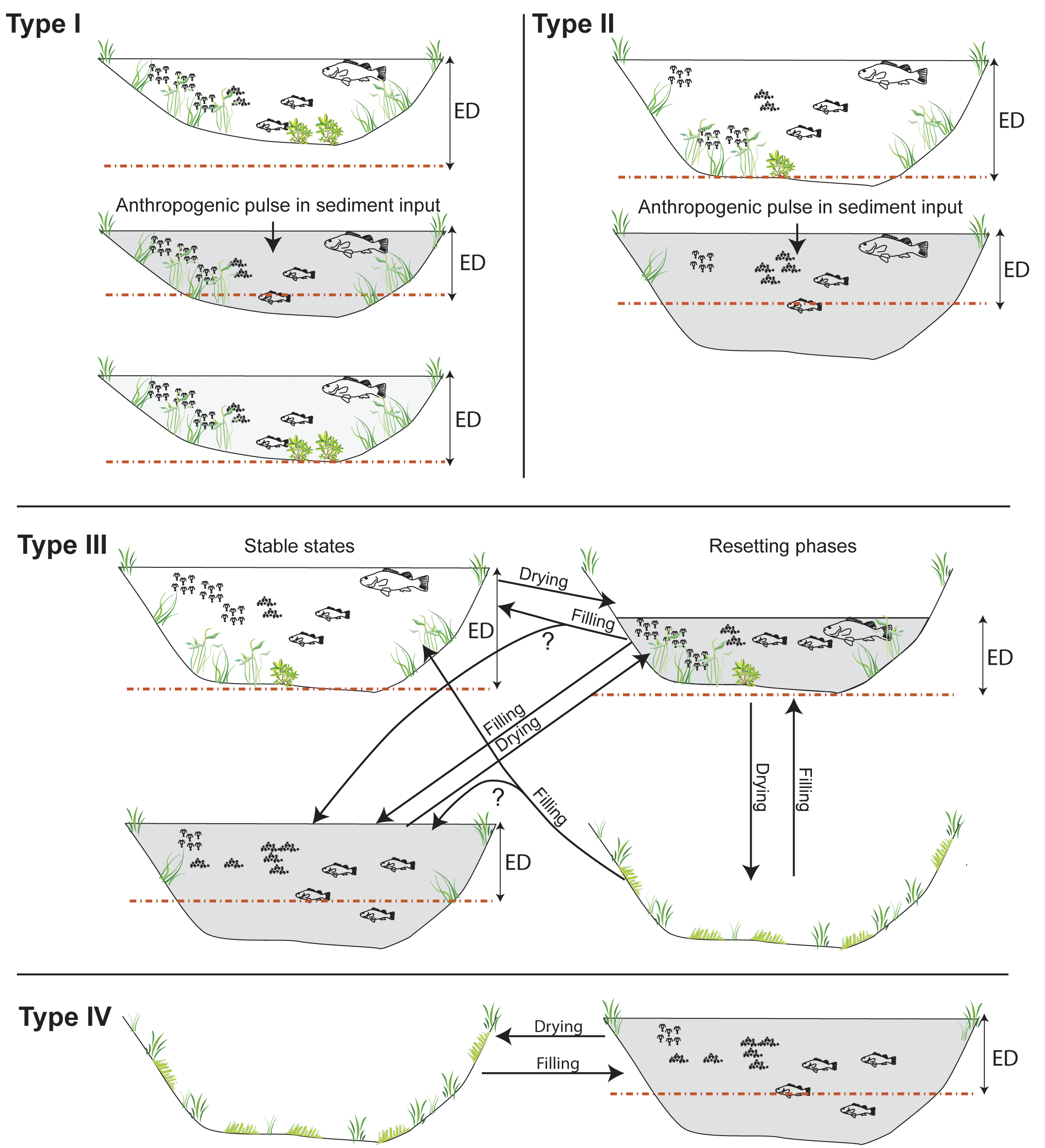
Figure 2: Conceptual models explaining the relationships between billabong geomorphology and hydrology and the proposed response types. In all types, dotted horizontal lines indicate the depth to which macrophytes could grow, ED = Euphotic Depth. Type I billabongs are resilient to reduced photic depth because pulses in anthropogenic sediment input do not result in reductions in photic depth sufficient to remove the majority of the billabong bed from the photic zone. Type II billabongs are less resilient to reduced photic depth because pulses in anthropogenic sediment input result in the removal of the majority of the billabong bed from the photic zone. In both cases, feedback processes act to strengthen the original (Type I) or new (Type II) state once sediment influx is reduced. Type III billabongs behave as Type II billabongs, but can be reset to either of the stable states by drying events. Type IV billabongs undergo frequent drying events and thus develop no stable states. |
Although there is site-to-site variation, analysis of the full suite of records suggests four broad response types exist (Fig. 2):
- Type I: where macrophyte-dominance persists throughout the record.
- Type II: where a switch from macrophyte to phytoplankton-dominance occurs, associated with European settlement.
- Type III: where periods of phytoplankton dominance occur before and after European settlement.
- Type IV: where there appears to be few periods of “stable” macrophyte or phytoplankton-dominance.
The nature of the changes varies across the southern basin and has a broad geographical pattern:
- Billabongs from Murray tributaries (Ovens, Goulburn and Murrumbidgee) tend to exhibit a Type I response.
- Billabongs from the middle Murray (between Hume Dam and the Murrumbidgee confluence) tend to exhibit a Type II response.
- Billabongs from between the Murrumbidgee and the Darling tend to exhibit a Type III response.
- Billabongs below the Darling tend to exhibit a Type IV response.
As the locations of sites in Figure 1 show, this pattern is not entirely consistent, particularly in the lower Murray. Nevertheless, the smaller channels of the Murray tributaries create smaller billabongs and hence a propensity for Type I responses. In contrast, the larger billabongs of the Murray are more susceptible to state changes in line with the model proposed by Ogden (2000). Further downstream, the drier climate and more variable hydrology introduces the potential for more frequent and extreme drying events. Thus, for billabongs exhibiting a Type III response, drying events may act to reset a new stable state once re-filling occurs. For billabongs exhibiting a Type IV response, drying phases may be too frequent for the establishment of strictly aquatic communities (planktonic or benthic) and hence these systems are dominated by opportunist taxa, such as amphibious or water tolerant terrestrial plants and algae, adapted to both benthic and pelagic habitats.
The broad geographical pattern suggests that the response types reflect the underlying geomorphology and hydrology of billabongs, because these features reflect the geomorphological and hydrological character of the parent river and reach. This understanding arises through the integration of a suite of site studies that enable the differentiation of site-specific change and regional drivers, and so provide evidence for management at a range of locations and management scales.
Implications
This regional synthesis allows for an assessment of the sensitivity of wetlands to catchment impacts and the status of groups of wetlands relative to their historical range of condition. For wetland managers, deep, large (Type II) wetlands are at risk yet smaller (Type I) wetlands reveal some resilience to catchment impacts. Lower down the system, armed with this evidence managers may better justify reinstating wetting-drying regimes to reset turbid wetlands provided sources of sediment are controlled. Lastly, for Type IV wetlands, this research shows that a “dry wetland” is an ecologically acceptable condition and regular artificial filling may not be justified. In all instances, this evidence reinforces notions that connectivity is key, but also that sediment flux remains a strong driver of wetland condition.
data
Metadata on the data presented in this article is available in the OZPACS database (http://www.aqua.org.au/Archive/OZPACS/OZPACS.html). The raw data are available on request from the author.
references
For full references please consult: http://pastglobalchanges.org/products/newsletters/ref2011_2.pdf
Chris R. Brodie1,2
1Department of Geography, Durham University, UK
2Department of Earth Sciences, Hong Kong University, Hong Kong: brodiehku.hk
Acid treatment of organic materials, necessary to remove inorganic carbon prior to isotopic analysis, adds an unpredictable and non-linear bias to measured C/N, δ13C and δ15N values questioning their reliability and interpretation.
C/N, δ13C and δ15N as paleoenvironmental proxies
The analysis of organic matter (OM) from modern and paleoenvironmental settings has contributed to the understanding of the carbon biogeochemical cycle at a variety of spatial and temporal scales. Specifically, the concentrations of carbon (C) and nitrogen (N), from which the C/N ratio is derived, and stable C and N isotopes (12C/13C, quoted as δ13C relative to Vienna Pee Dee Belemnite (V-PDB) and; 14N/15N, quoted as δ15N relative to N2-AIR) of OM have been used to understand processes from biological productivity through to paleoenvironmental interpretations. For example, C/N ratios are widely used as an indicator of OM origin (C/N < 10 interpreted as aquatic; C/N > 20 as terrestrial source) and δ13C can be used to, among other things, understand broad-scale changes in vegetation type (e.g., photosynthetic pathways; C3 and C4 plant types; Smith and Epstein, 1971; Meyers, 1997; 2003; Sharpe, 2007). δ15N has also been used to investigate OM origin (Thornton and McManus, 1994; Meyers, 1997; Hu et al., 2006), but is more commonly used to understand nitrate utilization, denitrification and N deposition in aquatic systems (e.g., Altabet et al., 1995). These interpretations are based on the assumption that we can reliably determine C/N, δ13C and δ15N values in OM.
Acid pre-treatment methods: The “free for all”
In the natural environment, carbon is commonly considered in two major forms—organic and inorganic (OC and IC). Both forms can act as a contaminant in the measurement of the other due to their distinctive isotopic signatures (e.g., IC is assumed to be enriched in 13C relative to OC: Hoefs, 1977; Sharpe, 2007). Therefore, the accurate determination of C/N and δ13C of OM necessarily involves the removal of IC from the sample material. This is commonly achieved by acid pre-treatment. A number of fundamentally different acid pre-treatment methods exist, within which a range of acid reagents and strengths, types of capsule and reaction temperatures are used. There is no consensus on “best practice”. An inherent, and widely unrecognized, assumption of these acid pre-treatment methods is that their effect on sample OM is either negligible or at least systematic (and small), implying that, within instrument precision, all measured values should be indistinguishable from one another regardless of the method followed. The type and strength of the acid reagent, and type of capsule the sample is combusted in, are assumed to have no effect on measured values. However, these assumptions have hitherto never been systematically investigated, implying that the scientific approach remains to be validated.
We examined three common acid pre-treatment methods for the removal of IC in OM: (1) Rinse Method: Acidification followed by sequential water rinse, the treated samples from which are combusted in tin (Sn) capsules (e.g., Midwood and Boutton, 1998; Ostle et al., 1999; Schubert and Nielsen, 2000; Galy et al., 2007); (2) Capsule Method: In-situ acidification in silver (Ag) capsules (e.g., Verardo et al., 1990; Nieuwenhuize et al., 1994a, b; Lohse et al., 2000; Ingalls et al., 2004); and (3) Fumigation Method: Acidification by exposure of the sample to an acid vapor in silver (Ag) capsules (e.g., Harris et al., 2001; Komada et al., 2008). δ15N is often measured from untreated sample aliquots weighed directly into Sn capsules, assuming negligible influence of inorganic nitrogen (e.g., Müller, 1977; Altabet et al., 1995; Schubert and Calvert, 2001; Sampei and Matsumoto, 2008). However, the application of “dual-mode” isotope analyses (the simultaneous measurement of C/N, δ13C and δ15N from the same pre-treated sample; e.g., Kennedy et al., 2005; Jinglu et al., 2007; Kolasinski et al., 2008; Bunting et al., 2010) is increasing. It was therefore also necessary to test whether acid pre-treatment had an effect on δ15N results. Hydrochloric (HCl), sulfurous (H2SO3) and phosphoric (H3PO4) acid, at varying strengths have been compared (e.g., Kennedy et al., 2005; Brodie et al., 2011a).
Non-linear, unpredictable bias to organic matter
 |
|
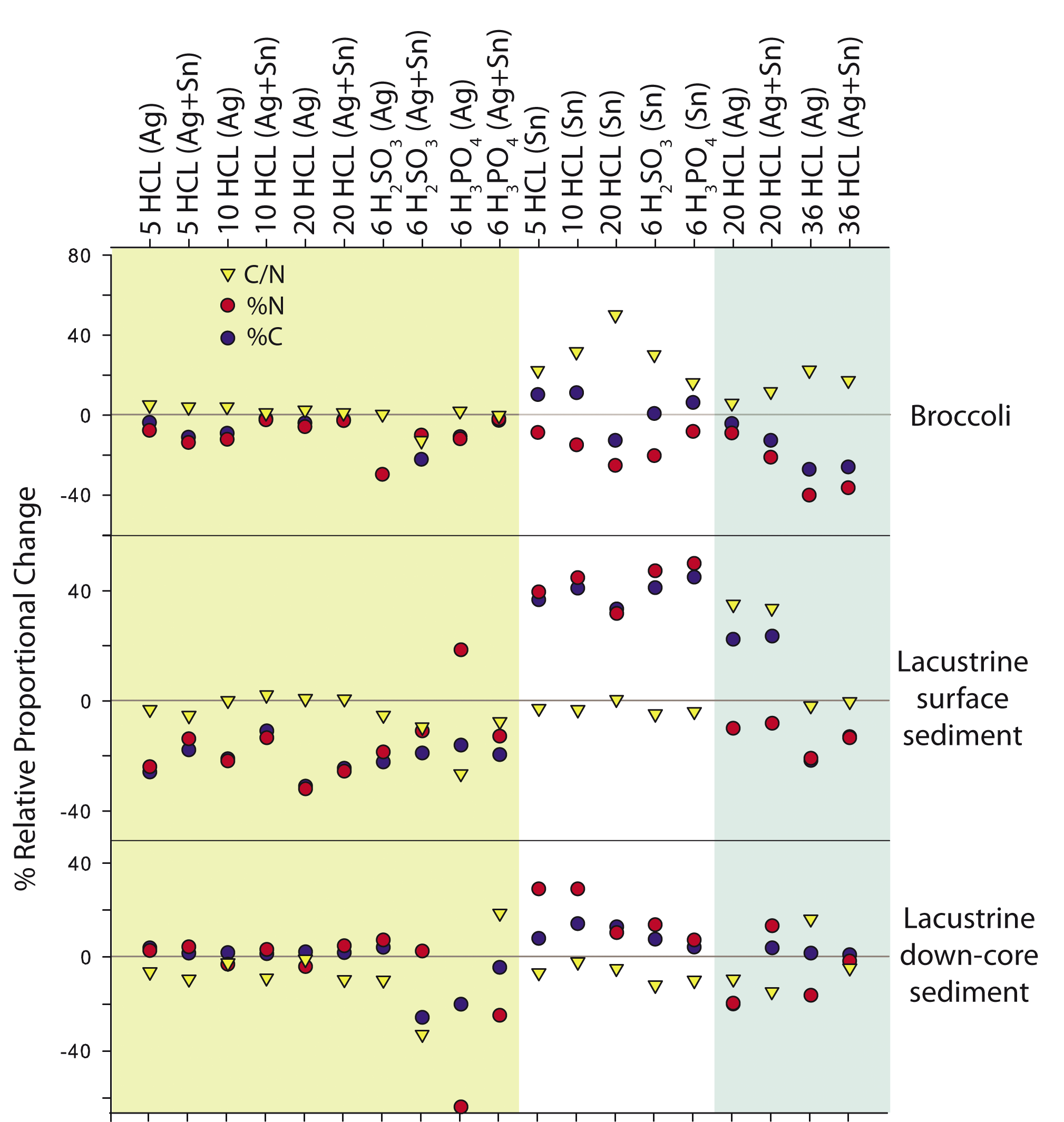
Figure 1: Relative offset in %C (blue circles), %N (red circles) and C/N (yellow triangles) for a selection of materials sampled (Details of additional samples in Brodie et al., 2011a), and all combinations of acid pre-treatment methods (varying concentrations of HCl, H2SO3 and H3PO4). Broccoli was calculated relative to known values. Of note, broccoli C/N results suggest either aquatic (<10) or aquatic/terrestrial (>10) origin. The lacustrine surface sediment (Newstead Abbey Lake, Nottingham, UK) and lacustrine down core sediment (Lake Tianyang, South China) were calculated relative to their overall means from all measured acidified samples. Background shading represents pre-treatment method: Yellow = capsule, white = rinse, green = fumigation (figure modified from Brodie et al., 2011a). |
 |
|
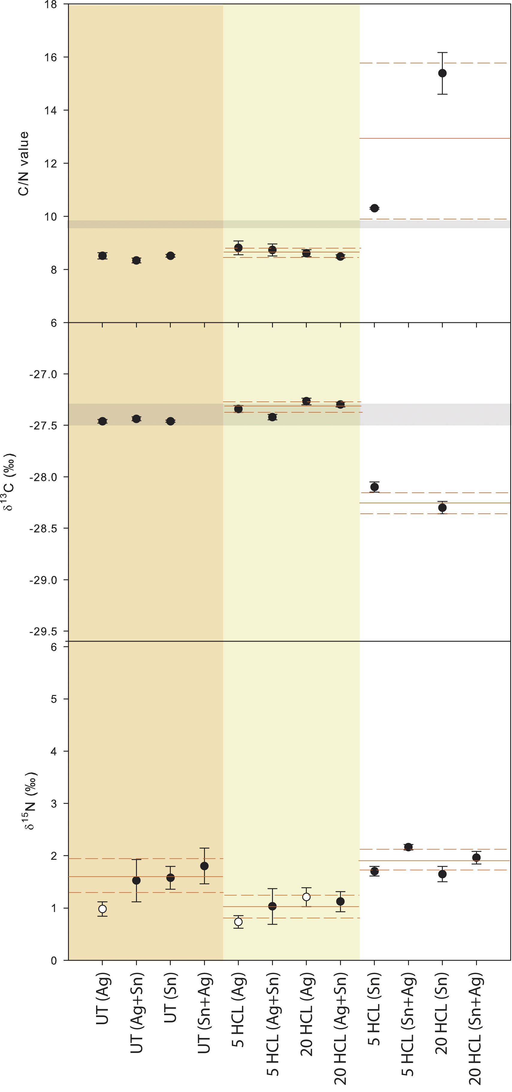
Figure 2: Broccoli C/N, δ13C and δ15N values for each pre-treatment method showing that measured C/N, δ13C and δ15N values vary in a non-linear, unpredictable manner within and between acid pre-treatment methods. Horizontal red lines indicate mean values for each method, and perforated red lines 1σ. Background shading represents pre-treatment method: Yellow = capsule, white = rinse, orange = untreated. Horizontal gray shaded bars represent known values. Error bars are calculated as standard deviation (1σ) of triplicate measurements. Unfilled circles represent samples analyzed in Ag capsules only (figure modified from Brodie et al., 2011b). |
Measured C/N, δ13C and δ15N values vary in a non-linear, unpredictable manner within (capsule type and acid reagent) and between (“capsule”, “rinse” and “fumigation”) acid pre-treatment methods (Fig. 1 and 2). In addition, the coherency of any one method or acid reagent is highly variable between the materials tested (i.e., high variability in accuracy and precision). This suggests that the measured C/N, δ13C and δ15N values of OM are not only dependent on environmental process, but also on analytical procedure, reducing the reliability of the data to the point of questioning the strength of the subsequent interpretation. Across all of the materials and pre-treatment methods tested, biases in C/N were in the range of 7 – 113; δ13C in the range of 0.2 – 7.1 ‰; and δ15N in the range of 0.2 – 1.5 ‰, resulting directly from bias to sample OM by acid treatment and in some instances residual IC (see Brodie et al., 2011a, b for a detailed discussion). The range and magnitude of these treatment-induced biases indicate that the assumption that there is negligible or systematic effect from acid pre-treatment is seriously flawed.
The range and magnitude of these biases are influenced by a number of factors. For example, %C and %N can be artificially concentrated by weight in the “rinse” method due to a loss a fine colloidal materials in the discarded supernatant; and C/N, δ13C and δ15N values can be biased due to loss of fine colloidal organic in the supernatant and solubilization of OC (Brodie et al., 2011a). These values can similarly be influenced in the “capsule” and “fumigation” methods due to volatilization of OC and residual IC. Furthermore, the type of acid reagent (e.g., HCl, H2SO3 or H3PO4) and strength of acid reagent (e.g., 5% HCl, 10% HCl or 20% HCl) within and between pre-treatment methods can affect the accuracy and precision of measured values. In addition, the capsule within which the sample is combusted can influence results due to the fundamental difference in combustion temperatures (Sn is 232°C and Ag is 962°C). Sample size, C and N homogeneity and the type, amount and nature of OM, can further influence the analysis. The underlying mechanisms causing these biases, however, remain unclear.
Implications for interpretation of C/N, δ13C and δ15N values
Bias by acid pre-treatment on OM can significantly undermine C/N values as indicators of OM provenance. For example, Figures 1 and 2 show that although broccoli (Brassica oleracea) is a terrestrial C3 plant, an aquatic or aquatic/terrestrial combination could be concluded from the data, depending upon the method and/or acid reagent (see Brodie et al., 2011a). In addition, C/N values can also vary considerably depending on whether they are calculated with %N from treated or untreated sample aliquots (see Brodie et al., 2011a, b). For δ13C, biasing in the range of 0.2 – 7.1‰ can undermine C3 vs. C4 plant type interpretations, and together with C/N undermine bi-plot interpretations of C/N, δ13C and δ15N values. This clearly demonstrates that the data are inherently unreliable as a function of the analytical approach. Although the underlying mechanisms require further research, it is clear the biases represented here across a range of terrestrial and aquatic, modern and ancient organic materials has direct implications for paleo reconstructions: understanding and reducing the uncertainty on the data is an essential prerequisite for reliable interpretations and reconstructions.
Concluding Remarks
The systematic comparisons of Brodie et al. (2011a, b) clearly demonstrate non-linear and unpredictable biasing of OM due to acid pre-treatment, and concomitantly indicate that complete IC removal (the purpose of acid pre-treatment) is not guaranteed. It is concluded that these biases are inherently not correctable but inevitable, and have a direct consequence for the accuracy and precision of measured values (i.e., significantly greater than instrument precision). Moreover, environmental interpretations of the data in both modern and paleo systems could be highly questionable.
acknowledgements
The author is grateful to J. Casford, J. Lloyd, Z. Yongqiang, T. Heaton, M. Bird and M. Leng for their support and discussions. Financial support came from the NERC through PhD studentship (NE/F007264/1), a NERC isotope Facility grant (IP/1165/0510), and the Dudley Stamp Memorial Fund.
references
For full references please consult: http://pastglobalchanges.org/products/newsletters/ref2011_2.pdf
Michael Zemp1, H.J. Zumbühl2, S.U. Nussbaumer1,2, M.H. Masiokas3, L.E. Espizua3 and P. Pitte3
1World Glacier Monitoring Service, Department of Geography, University of Zurich, Switzerland; michael.zempgeo.uzh.ch
2Institute of Geography and Oeschger Centre for Climate Change Research, University of Bern, Switzerland
3Argentine Institute of Snow Research, Glaciology and Environmental Sciences, (IANIGLA), CCT-CONICET Mendoza, Argentina
Reconstructions of glacier front variations based on well-dated historical evidence from the Alps, Scandinavia, and the southern Andes, extend the observational record as far back as the 16th century. The standardized compilation of paleo-glacier length changes is now an integral part of the internationally coordinated glacier monitoring system.
Glaciers are sensitive indicators of climatic changes and, as such, key targets within the international Global Climate Observing System (GCOS, 2010). Glacier dynamics contribute significantly to global sea level variations, alter the regional hydrology, and determine the vulnerability to local natural hazards. The worldwide monitoring of glacier distribution and fluctuations has been well established for more than a century (World Glacier Monitoring Service, 2008). Direct measurements of seasonal and annual glacier mass balance, which are available for the past six decades, allow us to quantify the response of a glacier to climatic changes. The variations of a glacier front position represents an indirect, delayed, filtered and enhanced response to changes in climate over glacier-specific response times of up to several decades (Jóhannesson et al., 1989; Haeberli and Hoelzle, 1995; Oerlemans, 2007). Regular observations of glacier front variations have been carried out in Europe and elsewhere since the late 19th century. Information on earlier glacier fluctuations can be reconstructed from moraines, early photographs, drawings, paintings, prints, maps, and written documents. Extensive research (mainly in Europe and the Americas) has been carried out to reconstruct glaciers fluctuations through the Little Ice Age (LIA) and Holocene (e.g., Zumbühl, 1980; Zumbühl et al., 1983; Karlén, 1988; Zumbühl and Holzhauser, 1988; Luckman, 1993; Tribolet, 1998; Nicolussi and Patzelt, 2000; Holzhauser et al., 2005; Nussbaumer et al., 2007; Zumbühl et al., 2008; Masiokas et al., 2009; Nesje, 2009; Holzhauser, 2010; Nussbaumer and Zumbühl, 2011). However, the majority of the data remains inaccessible to the scientific community, which limits the verification and direct comparison of the results. In this article, we document our first attempt towards standardizing reconstructed glacier front variations and integrating them with in situ measurement data of the World Glacier Monitoring Service (WGMS).
Standardization and database
The standardization of glacier front variations is designed to allow seamless comparison between reconstructions and in situ observations while still providing the most relevant information on methods and uncertainties of the individual data series. The standardized compilation of in situ observations is straightforward: the change in glacier front position is determined between two points in time and supplemented by information on survey dates, methods and data accuracies. The reconstruction of paleo-glacier front positions and their dating is usually more complex and based on multiple sources of evidence. Spatial uncertainty can arise from ambiguous identification of the glacier terminus, while temporal uncertainty is associated with the dating technique used in each case. A good example is the use of oil paintings, where it is important to distinguish between the time of first draft (e.g., a landscape drawing in the field) and production of the painting itself, which could happen several years later.
 |
|
Figure 1: Fluctuations of the Mer de Glace, France, during and following the LIA, reconstructed from a variety of sources (Nussbaumer et al., 2007). Length changes (relative to AD 1644 = maximum of LIA) were derived from documentary data as shown in the compilation below the x-axis, where small horizontal lines indicate uncertainties concerning the date of the document. Landmarks are indicated beside the y-axis. In situ measurements for the 1911–2003 period were obtained from the Laboratory of Glaciology and Geophysical Environment in Grenoble. Images a–d: The Mer de Glace (a) in 1804 drawn by Jean-Antoine Linck, (b) in 1842 mapped by James David Forbes, (c) in the 1850s photographed by Henri Plaut, and (d) in 2005 (Nussbaumer et al., 2007). |
The concept of integration of reconstructed front variations into the relational glacier database of the WGMS was jointly developed by natural and historical scientists. The glacier reconstruction data are stored in two data tables. The first table contains summary information of the entire reconstruction series including a figure of the cumulative length changes, investigator information, and references. The second table stores the individual glacier front variation data, minimum and maximum glacier elevation, and metadata related to the reconstruction methods and uncertainties. The metadata are stored in a combination of predefined choices of methods and open text fields. This ensures a standardized description of the data, but also provides space for individual remarks. Both data tables are linked by a unique numeric glacier identifier to the main table of the WGMS database with general information of the present-day glacier. This database relationship enables the direct comparison of reconstructed with observed front variations. Figure 1 shows an example for the Mer de Glace glacier with the sum of available meta-information stored within the database.
Results and discussion
 |
|
Figure 2: Reconstructed and measured cumulative glacier front variations in the Alps, Norway and southern South America since the Little Ice Age (LIA). The zero value on the y-axis corresponds to the most extensive front position of glaciers during the LIA. The period with direct front measurements is indicated by light green background. Gray vertical bars show the total number of available data for the selected glaciers. Note the significantly lower number of data points available from the Southern Andes. |
The WGMS database contains detailed inventory information of about 100,000 glaciers worldwide. In addition, in situ observations of frontal variations of 1,800 glaciers, mass balance data of 230 glaciers, and reconstructed frontal variations of the 26 glaciers mentioned below are now readily available in standardized and digital form. The reconstructed front variations extend the direct observations (mostly from the 20th century) by two centuries in Norway and by four centuries in the Alps and South America. Also available are moraines data back to the mid-Holocene. The direct comparison of long-term reconstructions with in situ observations reveals some striking features (Fig. 2).
The investigated glaciers in the western and central Alps show several periods of marked advances during the LIA, that are similar or even larger than LIA extent around AD 1850. Reconstructions reveal dramatic glacier advances that started in the late 16th century, overran cropland and hamlets, and reached maximum lengths at ca. AD 1600 and 1640 (Zumbühl, 1980; Nussbaumer et al., 2007; Steiner et al., 2008). Further maxima in glacier extent were reached around AD 1720, 1780, 1820 and 1850. After this last event, the direct measurement series show an impressive glacier retreat of 1-3 km, with intermittent minor re-advances in the 1890s, 1920s and between AD 1965 and 1985.
The historically based reconstructions for glaciers in southern Norway (Nussbaumer et al., 2011; Nesje, 2009) indicate that the maximum glacial extent of the LIA peaked around AD 1750 at Jostedalsbreen and in the late 1870s at Folgefonna. The reconstructed front variation series of Nigardsbreen (an outlet glacier of Jostedalsbreen) shows that the maximum LIA expansion occurred in AD 1748, and that it was preceded by a period of strong frontal advance that lasted (at least) 3-4 decades. Other sources report devastation of pastures by neighboring glaciers at that time (Nussbaumer et al., 2011). Direct observations at Nigardsbreen and other glaciers in southern Norway reveal a regional pattern of recent intermittent re-advances mainly during the 1990s. It is worthwhile to note that the extent of Nigardsbreen in the 17th century was similar to that of the present day (Nesje et al., 2008), and that the period of glacier re-advances in the 1990s is short (both in time and extension) considering the overall retreat of 1-4 km since the LIA maximum.
In southern South America, datable evidence for past glacier variations is most abundant in the Patagonian Andes. Despite recent efforts in this region and in other Andean sites to the north (Espizua, 2005; Espizua and Pitte, 2009; Jomelli et al., 2009; Masiokas et al., 2009), the number of chronologies of glacier fluctuations prior to the 20th century is still limited. In the southern Andes, most records indicate that glaciers were generally more extensive prior to the 20th century, with dates of maximum expansion ranging from the 16th to the 19th centuries. Based on the available evidence, Glaciar Frías (northern Patagonian Andes) probably contains the best-documented history of fluctuations since the LIA in southern South America, covering the period between AD 1639-2009.
Conclusions and outlook
Reconstructed LIA and Holocene glacier front variations are crucial for understanding past glacier dynamics and enable an objective assessment of the relative significance of recent glacier fluctuations (i.e., 20th and late 19th century changes) in a long-term context. The standardized compilation and free dissemination of reconstructed and in situ observed glacier fluctuation records offer several benefits for both data providers and users. Their incorporation within the international glacier databases guarantees the long-term availability of the data series and increases the visibility of the scientific results (which in historical glaciology are often the work of a lifetime). Furthermore, the database facilitates comparisons between glaciers and between different methods, and opens the field to numerous scientific studies and applications.
As the next steps of this new initiative, we aim to: (1) integrate a greater number of time series, (2) incorporate records that cover the entire Holocene, and (3) include data from other regions (e.g., the Himalayas, North America). Ideally, the growing new dataset will facilitate collaboration between the glacier monitoring and reconstruction communities and become an additional tool for the comparison of present-day to pre-industrial climate changes. This should eventually result in new scientific findings (e.g., related to the climatic interpretation of past and present glacier fluctuations).
International glacier databases: Requesting and submitting data
Worldwide collection of standardized data on the distribution and changes of glaciers has been internationally coordinated since 1894. Today, the World Glacier Monitoring Service (www.wgms.ch) is in charge of the compilation and dissemination of glacier datasets in close collaboration with the US National Snow and Ice Data Center (www.nsidc.org) and the Global Land Ice Measurement from Space initiative (www.glims.org) within the framework of the Global Terrestrial Network for Glaciers (www.gtn-g.org).
For available data or guidelines on data submission please check these websites and/or contact us directly: wgmsgeo.uzh.ch
acknowledgements
We are grateful to Wilfried Haeberli and Heinz Wanner for their valuable assistance. This work has been supported by the Swiss National Science Foundation (grant 200021-116354). The collection and processing of data from Argentinean glaciers was supported by Agencia Nacional de Promoción Científica y Tecnológica (grants PICT02-7-10033, PICT07-03093 and PICTR02-186), and the Projects CRN03 and CRN2047 from the Inter American Institute for Global Change Research (IAI).
references
Nussbaumer, S.U., Zumbühl, H.J. and Steiner, D., 2007: Fluctuations of the Mer de Glace (Mont Blanc area, France) AD 1500–2050: an interdisciplinary approach using new historical data and neural network simulations, Zeitschrift für Gletscherkunde und Glazialgeologie 40(2005/2006): 1-183
WGMS, 2008: Global Glacier Changes: facts and figures, Zemp, M., Roer, I., Kääb, A., Hoelzle, M., Paul, F. and Haeberli, W. (Eds.), UNEP, World Glacier Monitoring Service, Zurich, Switzerland, 88 pp
Zumbühl, H.J., 1980: Die Schwankungen der Grindelwaldgletscher in den historischen Bild- und Schriftquellen des 12. bis 19. Jahrhunderts. Ein Beitrag zur Gletschergeschichte und Erforschung des Alpenraumes, Denkschriften der Schweizerischen Naturforschenden Gesellschaft (SNG), Band 92. Birkhäuser, Basel/Boston/Stuttgart, 279 pp
For full references please consult: http://pastglobalchanges.org/products/newsletters/ref2011_2.pdf
Thomas J. Crowley
Braeheads Institute, Maryfield, Scotland, UK; tcrowley111googlemail.com
The Brazil Current may have played a key role in shunting heat towards the Antarctic during the meridional overturning shutdown at the end of the last ice age.
The remarkable relationship between late Pleistocene carbon dioxide variations and Antarctic temperatures has been as inscrutable as the faint smile of a stone Buddha. Recently, a string of papers provide promise of unlocking the secrets of that relationship by shedding light on ocean circulation/carbon dynamics involving the key first phase of carbon dioxide rise at the end of the last glacial period. During an interval that has long been termed the “Late Glacial”, and is broadly correlative with Heinrich Event 1 (H1, ~17.8-14.6 cal ka), significant carbon reservoir changes at the time of the first major CO2 rise have been related to Antarctic ocean circulation changes (Marchitto et al., 2007; Anderson et al., 2009; Rose et al., 2010). In turn, these changes link to variations in North Atlantic Deep Water (NADW) overturning rate (Anderson et al., 2009; Toggweiler and Lea, 2009), which cause a see-saw in sea surface temperature (SST) patterns between the North and South Atlantic (Crowley, 1992; Toggweiler and Lea, 2009).
 |
|
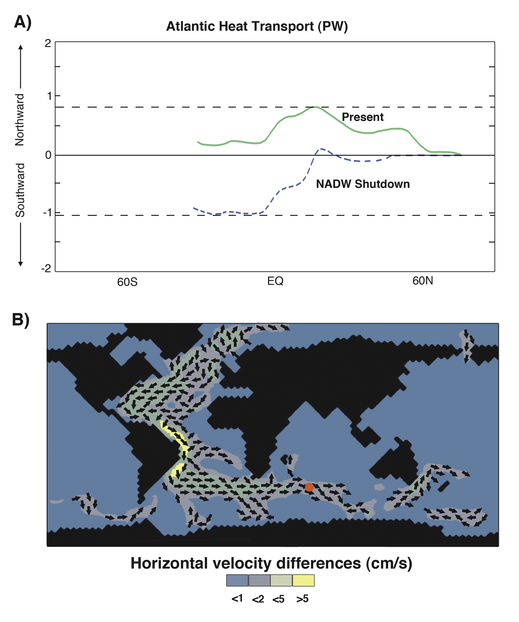
Figure 1: A) Comparison of zonal poleward ocean heat transport (1 PW = 1015 Watts) in the Atlantic sector for the model runs illustrated in Figure 2. Figure from Maier-Reimer et al., 1996. B) Difference of surface current (25 m) between the control and perturbed run, illustrating the effects of an NADW shutdown (in this case due to an open central American isthmus) on global ocean circulation (Figure from Maier-Reimer et al., 1990). Red dot refers to location of sub-Antarctic core illustrated in Figure 2. |
In this note, I point out that an overlooked feature of the NADW see-saw provides additional insight into the nature of the “bolt of warmth” that characterized Antarctic temperature change at this time. As noted in Crowley (1992), shutdown of NADW production “banks” about 1 petawatt (PW) of heat in the South Atlantic, which would otherwise be exported north of the equator to compensate for southward outflow of NADW across the equator. An early modeling study indicates that adjustment of the South Atlantic to this shutdown involves an enormous 1 PW increase in heat transport (Maier-Reimer et al., 1990; Fig. 1A), which is shunted southward into higher latitudes via the Brazil Current, i.e., the western boundary surface current of the South Atlantic (Fig. 1B).
It is remarkable that the South Atlantic model heat transport for the perturbation run is greater than for the Gulf Stream in the control run (Fig. 1A). In a sense the deglacial Brazil Current vertical section and transport is dynamically similar to the Gulf Stream at present—the strong flow is required to compensate for both the increased northward transport of Antarctic Bottom Water and the decreased southward transport of both NADW and North Atlantic Intermediate Water. Enhanced Southern Ocean inflow into Atlantic Basins is supported by geochemical assays (Negre et al., 2010).
 |
|
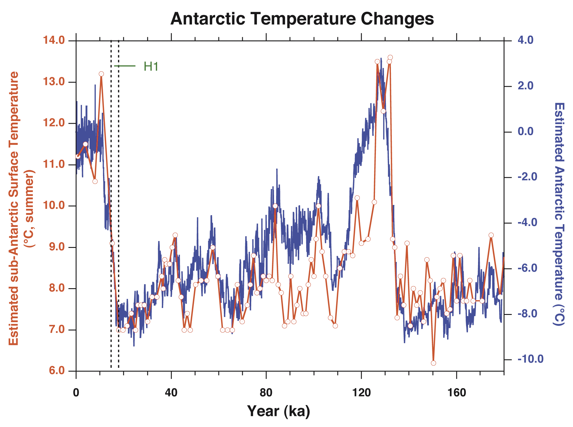
Figure 2: Comparison of the sub-Antarctic record (core RC11-120; Hays et al., 1976), using higher-resolution sampling from Martinson et al. (1987) and converted to an updated marine chronology (Lisiecki and Raymo, 2005), with the Vostok deuterium isotope record and ice core GT4 chronology (Petit et al., 1999). H1 interval is Heinrich Event 1. |
In the illustrated model example, convergence of the stronger Brazil Current with sub-Antarctic waters leads to stronger currents (Fig. 1B) and presumably enhanced convergence in the frontal zone (cf., Marchitto et al., 2007), with changes extending zonally downstream at least as far as the eastern Indian Ocean. These changes are likely responsible for the observed zonal changes in the Antarctic Circumpolar Current (cf., Anderson et al., 2009). The heat injection, along with a sea-ice melt feedback, likely explains the long-known (Hays et al., 1976) rising temperatures in the sub-Antarctic at the time of H1 (e.g., Fig. 2), and the parallel rise recorded in Antarctic ice cores. Additional adjustments can be expected from the warming effects of surface warming on the Antarctic overturning circulation, with potential implications for possible tapping of the deeper ocean glacial carbon reservoir in the Southern Ocean (Toggweiler and Samuels, 1995; Rose et al., 2010). It is conceivable that warmer surface waters could have prevented recharge of very cold and saline deep Antarctic waters, leading to a transient enhanced vertical stratification (tidal mixing would probably break down this barrier after a few hundred years; R.-X. Huang, pers. comm.).
It therefore appears that the Brazil/Malvinas-Falkland Convergence (where the southerly vectors of the Brazil Current merge with the easterly flow of the Subantarctic in Figure 1B) may be the pressure point where the heat accumulated in response to stalled Atlantic overturning circulation is injected into southern high latitudes, thereby driving the planet into deglaciation through positive feedbacks from ocean-circulation releasing carbon stored in the deep ocean around Antarctica. Closer inspection of data from the Malvinas/Falkland region might provide enhanced insight into kinematics of this process. The postulated response should also be testable with the present generation of coupled climate/carbon models and would be much more realistic if started from a glacial base state. The transient model response would be especially intriguing to examine, for it could provide fascinating insight into the time-space evolution of the heat package injected into the sub-Antarctic region and the partitioning of the heat between the ocean and the atmosphere (Seager et al., 2002).
Even though the model results invoked herein represent an uncoupled run from twenty years ago, I suggest that the system response is so constrained by conservation of volume arguments—overturning shutdown in the north blocking heat export from the South Atlantic—that newer model simulations are likely to respond in the same manner. Elements of this argument can even be traced back to (or at least anticipated in) Henry Stommel’s classic explanation for differences in strength of the Gulf Stream and Brazil Current (Stommel, 1965). His interpretation was certainly supported by the 1990 simulation (Maier-Reimer et al., 1990).
data
Data for Fig. 2 from Martinson et al. (1986) and NOAA/NGDC Paleoclimatology website.
references
For full references please consult: http://pastglobalchanges.org/products/newsletters/ref2011_2.pdf
Nicholas Graham1 and Eugene Wahl2
1Hydrologic Research Center, and Scripps Institution of Oceanography, USA; ngrahamhrc-lab.org
2NOAA, National Climatic Data Center, Paleoclimatology Branch/World Data Center for Paleoclimatology, Boulder, USA
The last millennia Paleoclimate Reconstruction (PR) Challenge is a model-based venue for experimenting with climate reconstruction methods. The overall idea has been described before (Ammann, 2008) and a modified version of the Challenge is now "live" and available for participation. It is designed to engage the scientific paleoclimate community in examining its methods in a common framework for the purpose of evaluating their relative strengths and weaknesses. A key design element of the Challenge is to allow true "apples to apples" comparison of reconstruction methods across identical experimental platforms. The ultimate goal is to improve last two millennia PR methods so that paleoclimate science can offer the best possible information to help understand both natural and anthropogenic climate change.
The Challenge is organized around 4 themes. In each theme, a set of long (1,000+ yrs) forced global climate model (GCM) integrations is used to formulate simulated paleoclimate proxy data (pseudo-proxies) and to provide pseudo-instrumental climate data for calibration and examination of reconstruction fidelity. Several different GCM runs provide a range of simulated climate evolutions that present different reconstruction scenarios. In each Theme, the reconstruction method used is at the prerogative of the participants.
Theme 1: Reconstruction of Northern Hemisphere temperature with strongly limited proxy data set (implemented)
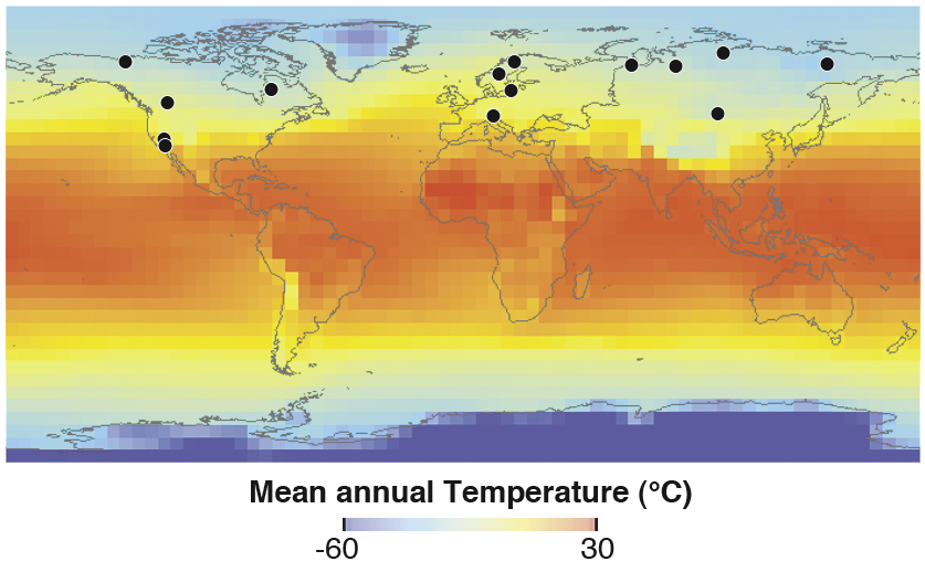 |
|
Figure 1: Map showing the location of the 14 simulated extratropical tree-ring-chronology sites (black dots) in the Northern Hemisphere that were used in Theme 1 for the reconstruction of Northern Hemisphere temperature with strongly limited proxy data set. Underlying colors represent average annual temperatures (1961-1990). Figure by W. Goss, NOAA-NCDC Paleoclimatology/WDC for Paleoclimatology). |
This theme focuses on the capacity of a very limited set of proxy data sites to enable reconstruction of hemispheric (20-90° N) mean annual temperature. The pseudo-proxy data-set consists of 14 extratropical tree-ring-chronology sites in the Northern Hemisphere (Fig. 1). It is designed to mimic the dataset used by Esper et al. (2002).
Theme 2: Reconstruction of Northern Hemisphere temperature and spatial patterns with a richer, but still somewhat limited proxy data set (in process of implementation)
This theme focuses on the capacity of a less limited set of proxy-data sites to enable reconstruction of hemispheric (again defined as 20-90°N) mean annual temperature and spatial temperature patterns. The pseudo-proxy data set consists of 66 tree-ring sites in the Northern Hemisphere at >40°N and is designed to mimic the dataset used by D'Arrigo et al. (2006).
Theme 3: Reconstruction of Northern Hemisphere temperature and global spatial patterns using a relatively rich proxy data set (to be implemented)
This theme focuses on the capacity of a richer and more spatially diverse set of proxy data sites to enable reconstruction of hemispheric (here defined as 0-90°N) mean annual temperature and global spatial temperature patterns. The pseudo-proxy data set contains 104 sites from different archives spread across the globe. It is designed to mimic the dataset used by Mann et al. (1998) and in numerous reconstruction simulation experiments (e.g., Mann et al., 2007; Smerdon et al., 2010).
The above three themes are designed to explore how proxy richness and spatial extent affect reconstruction fidelity of the Northern Hemisphere mean temperature (Themes 1-3), and of spatial temperature patterns in the Northern Hemisphere (Theme 2) and globally (Theme 3).
Theme 4: Reconstruction of spatial drought patterns (currently in development)
This theme is still under development; it will be based on a pseudo-proxy dataset designed to mimic that used in the North American Drought Atlas (NADA; cf., Cook et al., 2004). A timetable for implementation is being developed.
The Paleoclimatology Branch of NOAA's National Climatic Data Center/World Data Center for Paleoclimatology is providing the simulated proxy and instrumental data sets of the PR-Challenge and is also archiving the contributed reconstructions so that they can be cross-compared: www.ncdc.noaa.gov/paleo/pubs/pr-challenge/pr-challenge.html.
The PR-Challenge implementation team consists of Nicholas Graham, Rosanne D'Arrigo, Kevin Anchukaitis, Eugene Wahl, and David Anderson. We gratefully acknowledge Edward Cook for valuable ideas and encouragement, and Caspar Ammann for his inception of the PR Challenge project. Tree-ring pseudo-proxy formulation used the "VS-Lite" tree growth model developed by Suz Tolwinski-Ward and collaborators (Tolwinski-Ward et al., 2010).
The PR-Challenge is sponsored by NOAA's Office of Oceanic and Atmospheric Research/Climate Program Office (Climate Change Data and Detection Program, grant NA08OAR4310732) and the PAGES/CLIVAR Intersection.
references
Amman, C., 2008: The Paleoclimate Reconstruction Challenge, PAGES news 16(1): 4
For full references please consult: http://pastglobalchanges.org/products/newsletters/ref2011_2.pdf
Sami Hanhijärvi
Department of Environmental Sciences, University of Helsinki, Finland; sami.hanhijarvihelsinki.fi
Meeting of the PAGES Arctic2k Working Group – San Francisco, USA, 11-12 December 2010
The Arctic has witnessed increased warming in comparison to other parts of the globe. Due to this amplification, the Arctic is a key region for climate studies, and is potentially central in elucidating the processes that govern the 19th and 20th century global warming. The PAGES Arctic2k Working Group was initiated to research the climate of the Arctic region within the past 2000 years. The Working Group had its second meeting in San Francisco, which was attended by 10 participants.
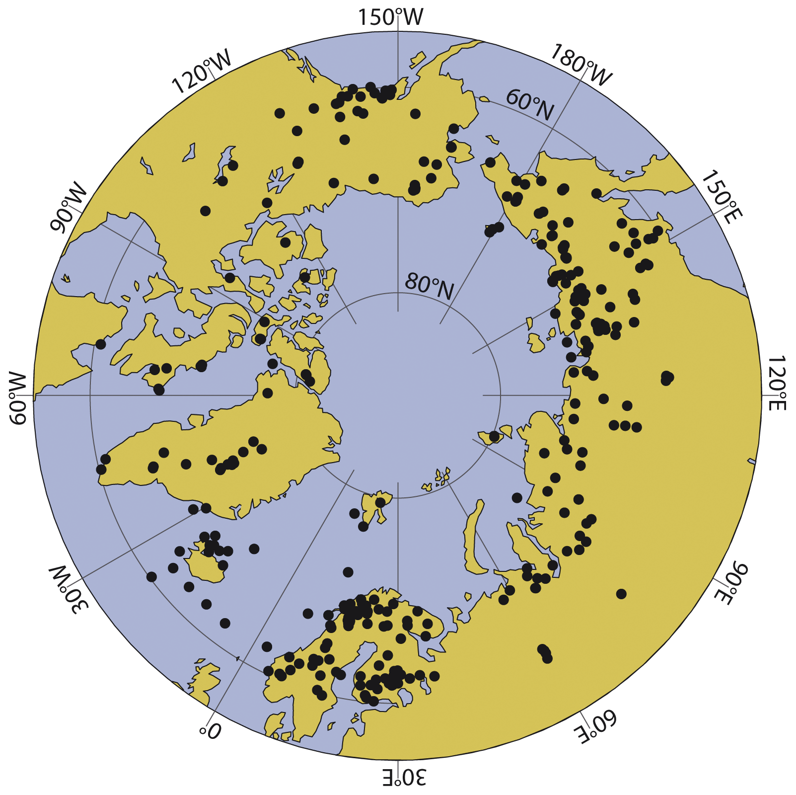 |
|
Figure 1: Spatial coverage of proxy records that extend back to 1500 AD in the Arctic. Proxy locations are a combination from Mann et al., 2008; Kaufman et al., 2009; Ljungqvist, 2010; Sundqvist et al., 2010; and from the NOAA Paleoclimatology database. |
To date, much of the Working Group’s efforts have been focused on generating high quality, high-resolution proxy records from the Arctic region. At this meeting, a new Icelandic glacier proxy record was introduced in addition to a new type of ice cover proxy record. The group has also aspired to collect a comprehensive list of available records and information about their nature and quality. Figure 1 depicts the combined locations of proxy records used in recent multiproxy studies, as well as records available from the NOAA Paleoclimatology database.
The criteria for the inclusion of specific proxy records were thoroughly discussed and formulated to ensure selection of only high quality proxy records, to avoid swamping the collection and synthesis processes with low quality records. It was decided that the criteria and template for proxy metadata should be offered to other PAGES 2k Regional Groups, so that if adopted, the proxy lists of all 2k Regional Groups would be compatible and the collection efforts need not be replicated for a global synthesis.
The statistical problems of climate reconstructions were also discussed. The proxy records tend to be spatially clustered, which can cause over-representation of the clustered areas in the synthesis. Another problem discussed is that the proxy records do not directly record a certain climate parameter and transforming the proxy data to, for example, temperature is often not straightforward. Existing reconstruction methods were briefly listed and their assumptions were discussed.
The temporal uncertainty was identified as possibly the largest cause of uncertainty in proxy reconstructions. As annually resolved proxies do not have the necessary temporal and spatial coverage, proxies with uncertain dates are necessary for the inference of climate parameters, especially before 1000 AD. The temporal uncertainty has to be accounted for in the overall uncertainty of climate reconstructions, which poses methodological problems.
A number of scientific questions emerged during the workshop, ranging from the spatiotemporal patterns of the Arctic climate to the utilization of the future synthesis produced by the Working Group. The questions were subdivided into four milestones that form the outline of future research. The first milestone involves inferring the spatial and temporal variability of the Arctic climate, and how they relate to the instrumental records of the recent past. The second milestone tackles the abrupt events recorded in the history of the Arctic, with special focus on the frequency of such events and to the possible thresholds that were exceeded before these events. The third milestone combines the knowledge of the two previous ones and seeks to answer questions about the long-term modes of the Arctic climate variability, and how much of the variability can be explained by internal adjustment of the climate system versus the external forcings (such as changes in solar irradiance and volcanic activity). The final milestone aims at involving people from the climate modeling community to use the obtained results to improve and enhance the climate models and to increase the accuracy of future predictions.
references
Contributors of the IGBP PAGES/World Data Center for Paleoclimatology, NOAA/NCDC Paleoclimatology Program, Boulder, Colorado, USA