PAGES Magazine articles
Eduardo Leorri and David Mallinson
Department of Geological Sciences, East Carolina University, Greenville, USA; leorrie ecu.edu
Coastal changes have occurred throughout geological time due to tectonic and isostatic processes as well as sea level changes induced (primarily) by climatic changes. During the Quaternary, one of the main controls on coastal evolution was sea-level changes through the exchange of mass between ice sheets and oceans. However, local and regional changes are superimposed on the global signal. These local/regional changes become more important as the temporal scale resolution increases, producing substantial spatial and temporal variability in sea-level changes, even when localities lie close to each other. This becomes even more complex as humans occupied the coastal zone (e.g. Syvitski, this issue).
Furthermore, it seems that the overall warming and sea-level rise of the Holocene was punctuated by climatic events and, apparently, impacted the coastal evolution. In fact, a correlation between marsh evolution and rapid climatic changes (RCCs) in the Delaware Bay has been established at a millennial scale. The idea of coastal evolution linked to climatic changes is supported by stratigraphic sequences occurring simultaneously with RCCs recognized in the western Gulf of Mexico, in the Trinity/Sabine River incised valley system and in northern Spain. Among the RCCs identified during the Holocene, an event at 750-950 AD was characterized by polar cooling, tropical aridity and major atmospheric circulation changes. Although this event was global in scale, records of it are poorly correlated due to its different behavior between regions (Mayewski et al. 2004).
 |
|
Figure 1: A) Map of the Pamlico estuarine system in North Carolina showing the location of the main active inlets. B) Paleoenvironmental reconstruction of the southern Pamlico Sound region ca. 850 AD (modified from Grand Pre et al. 2011). Barrier island destruction along the southern Outer Banks resulted in a shallow, submarine sand shoal and localized deeper tidal channels over which normal marine waters were advected. The Cape Hatteras region exhibited several inlets with large flood-tide deltas. |
Concomitant with these reported RCC events, major coastal geomorphological changes have been identified. For instance, recent work undertaken in the US North Carolina estuaries and barrier islands suggests that the period ca. 750-1400 AD was characterized by a high degree of barrier island segmentation and open marine influence in areas now occupied by the modern estuaries. Figure 1B shows the interpretation of the environmental change that occurred in the southern part of the Pamlico Sound at 850 AD, reflecting the destruction of large segments of the barriers compared to the current situation (Fig. 1A) (Grand Pre et al. 2011). Estuaries along the southern Bay of Biscay reflect similar changes associated with RCCs. These changes might have impacted the tidal frame, currents and sediment transport. In fact, dramatic changes in the tidal frame have been modeled for the Bay of Fundy in response to the catastrophic breakdown of a barrier system (Shaw et al. 2010). Also, tidal changes have been recorded in Delaware Bay over the last 4000 years in response to the change of the basin shape during the late Holocene sea-level rise (Leorri et al. 2011).
Over the Holocene, coastal environments have moved across the landscape. However, accelerated rates of climate change and sea-level rise could affect coastal environments by overcoming the natural mechanisms of self-maintenance. The impact of these changes might be considered significant since there are more than 20,000 km of barrier islands along the world’s open ocean coast, and they represent the front line to impacts of projected climate change. This may alter coastal systems from current conditions in a number of ways by: 1) increasing salt water intrusion landward, producing more rapid salinization; 2) altering the species composition through modified migration and other mechanisms; 3) enhancing tidal erosion, potentially forcing a coastal retreat; and 4) increasing the potential impact of future storms.
In the case of North Carolina, it has been suggested that hurricanes impacted the barrier islands at ca. 850 AD, causing the destruction of large segments of barriers. These barrier destruction events are essentially synchronous with intervals of RCCs at 750-950 AD and are coincident with transgressive surfaces in Delaware Bay, highlighting the importance of environmental changes in coastal evolution and suggesting their potential impact for future coastal evolution.
acknowledgements
NSF (OCE-1130843); MICINN (CGL2009-08840), FCT (PTDC/CTE/105370/2008). IGCP Project 588.
selected references
Full reference list online under: http://pastglobalchanges.org/products/newsletters/ref2012_1.pdf
Grand Pre C et al. (2011) Quaternary Research 76, 319-334
Leorri E, Mulligan R, Mallinson D and Cearreta A (2011) Journal of Integrated Coastal Zone Management 11(3): 307-314
Mayewski PA et al. (2004) Quaternary Research 62: 243-255
Shaw J et al. (2010) Canadian Journal of Earth Science 47: 1079-1091
Jean-Pierre Gattuso
CNRS and Université Pierre et Marie Curie, Villefranche-sur-Mer, France; gattusoobs-vlfr.fr
 |
|
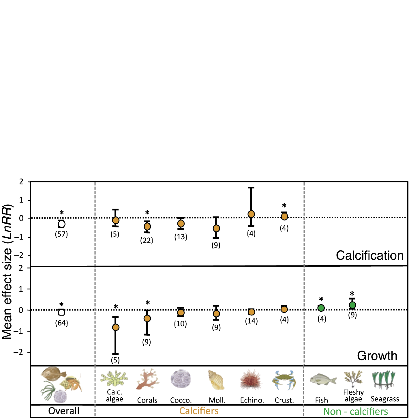
Figure 1: Effects of ocean acidification on marine organisms. Mean effect size and 95% bias-corrected bootstrapped confidence interval are shown. The number of experiments used to calculate mean effect sizes are shown in parentheses. Asterisks (*) mark significant mean effect sizes (95% confidence interval does not overlap zero). Figure adapted from Kroeker et al. (2010). |
Ocean acidification, an expression coined in the early 2000s, describes changes in the chemistry of seawater generated by the uptake of anthropogenic carbon dioxide (CO2). Among those changes is an increase in the concentration of dissolved inorganic carbon as well as a decrease in pH and the saturation state of calcium carbonate (Ω). Evidence for ocean acidification and its consequences for marine organisms and ecosystems have only recently begun to be investigated (Gattuso and Hansson 2011).
Some aspects of ocean acidification, such as the changes in the carbonate chemistry, are known with a high degree of certainty. It is also well established that three areas of the global ocean are more susceptible to ocean acidification than others, either because ocean acidification will be more severe (e.g. polar regions and the deep sea) or because it acts synergistically with another major stressor (e.g. coral reefs which are also strongly affected by global warming). Most biological, ecological and biogeochemical effects are much less certain. Calcification, primary production, nitrogen fixation and biodiversity will all be affected, but the magnitude of the projected changes remains unclear.
Although some studies indicate no effect or a positive effect of ocean acidification on the rate of calcification of some organisms (Andersson et al. 2011; Riebesell et al. 2011), meta-analyses reveal an overall significant, negative effect (e.g. Hendriks et al. 2010; Kroeker et al. 2010). In general, corals experience particularly adverse effects, whereas crustaceans, for example, grow thicker shells. Whether or not calcification decreases in response to elevated CO2 and lower Ω, the deposition of calcium carbonate is thermodynamically less favorable under such conditions. Some organisms could up-regulate their metabolism and calcification to compensate for lower Ω, but this would have energetic costs that would divert energy from other essential processes, and thus may not be sustainable in the long term. Full or partial compensation may be possible in certain organisms if the additional energy demand required to calcify under elevated CO2 can be supplied. We need to know much more about the molecular and physiological processes involved in calcifying marine organisms to better understand the response of calcification to ocean acidification.
Ocean acidification is expected to affect not only single organisms but whole populations and thus ecosystems. There is mounting evidence, especially for benthic communities, suggesting that their composition will change as the oceans acidify. For example, the structure of an ecosystem around submarine CO2 vents in the Mediterranean Sea appears to be governed by the concentration gradient around the vents (Barry et al. 2011). Non-calcareous algae replace calcareous ones closer to the vents, and no juvenile calcifiers are found close to the vents.
We know considerably less about the effects on composition of pelagic communities. Experiments on natural phytoplankton assemblages consistently show a modest increase in carbon fixation at elevated pCO2 (Riebesell and Tortell 2011). The increased CO2 levels would aid the growth of some groups of phytoplankton such as cyanobacteria, and decrease the competitiveness of others (e.g. some calcifiers). The combined effects of acidification and other global changes on ecosystems are uncertain but deserve more scrutiny, especially because of potential economic consequences on, for example, the fishing and tourism industry.
Ocean acidification and its impacts on marine ecosystems could provide an additional reason for reducing CO2 emissions, but we need to reduce the uncertainties and offer a prognosis despite the sometimes conflicting observations. Synthetic studies will be key to make sense of the many dimensions of ocean acidification and its interactions with other stressors such as warming, coastal eutrophication and deoxygenation. There is reason to be optimistic, at least on the research front: the coming years will witness the launch of major research initiatives, in addition to IPCC and other assessments, which are expected to considerably improve our level of understanding.
selected references
Full reference list online under: http://pastglobalchanges.org/products/newsletters/ref2012_1.pdf
Gattuso J-P et al. (2011) Ocean acidification: knowns, unknowns and perspectives. In: Gattuso J-P and Hansson L (Eds) Ocean acidification, Oxford University Press, 291-312
Gattuso J-P and Hansson L (2011) Ocean acidification: background and history. In: Gattuso J-P and Hansson L (Eds) Ocean acidification, Oxford University Press, 1-20
Hendriks IE, Duarte CM and Alvarez M (2010) >Estuarine, Coastal and Shelf Science 86:157-164
Kroeker K, Kordas RL, Crim RN and Singh GG (2010) Ecology Letters 13: 1419-1434
Riebesell U and Tortell PD (2011) Effects of ocean acidification on pelagic organisms and ecosystems. In: Gattuso J-P and Hansson L (Eds) Ocean acidification, Oxford University Press, 99-121
Ellen Thomas1,2
1Department of Geology and Geophysics, Yale University, New Haven, USA; ellen.thomasyale.edu
2Department of Earth & Environmental Sciences, Wesleyan University, Middletown, USA
 |
|
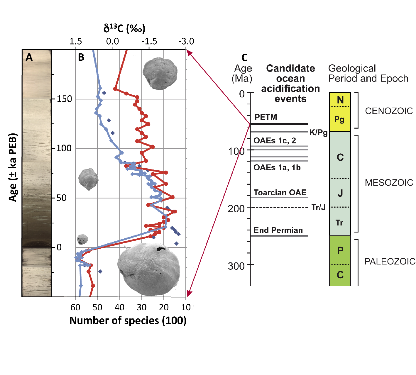
Figure 1: The Paleocene-Eocene Thermal Maximum at Walvis Ridge in the southeastern Atlantic Ocean, off Namibia. Paleo-water depth ~1500 m. A) Core image shows carbonate ooze (light colors) and clay (dark colors), where carbonate has been dissolved during ocean acidification (Zachos et al. 2005). Sediment is plotted on an age scale in ka relative to the Paleocene-Eocene Boundary (PEB) (Hönisch et al., in press). B) Blue curve and blue dots show carbon isotope excursion (CIE) in shells of deep-sea benthic foraminifera (McCarren et al. 2008). Red curve shows decrease in number of species of deep-sea benthic foraminifera during extinction coeval with CIE (Thomas, unpublished data). Pictures show specimens of the benthic foraminifer Nuttallides truempyi, used for isotope analysis, survivor of the extinction. All at the same magnification, showing severe decrease in size during ocean acidification, placed at the location where they occurred in the sediment. C) Climate-carbon cycle disturbance in the oceans during the last 300 Ma of Earth history (modified after Kump et al. 2009). |
Scientists use the geological record to ”look back into the future”, i.e. to evaluate effects of ocean acidification on whole marine ecosystems during carbon cycle-climate perturbations (Pelejero et al. 2010). Fortuitously, calcifying organisms, affected most immediately by decreased carbonate saturation (Fig. 1), have left a fossil record: planktic foraminifera and calcareous nannoplankton (coccolithophores) provide information on the effects of ocean acidification on calcifiers in surface oceans, benthic foraminifera and ostracodes in the deep sea, and corals, calcareous algae, echinoderms, bivalves and gastropods in shelf environments (Kiessling and Simpson 2011).
Where in the past can we find clues about future ocean acidification? To look at a world with CO2 levels higher than today (>389 ppm) we need to go back into “Deep Time” (Kump et al. 2009; NRC 2011). During transitions from glacial to interglacial periods over the last 2.6 million years (Ma), atmospheric CO2 levels increased by ~90 ppm over a few thousand years, but from ~175 to ~185 ppm, i.e. well below present levels. Atmospheric CO2 levels may not have been above ~400 ppm for the last 35 Ma, the time since when ice sheets existed on Antarctica. The Deep Time warm worlds are not perfect analogs for the near future, among other reasons because life has evolved since then, but nevertheless may provide useful insights.
The long-term high pCO2 and low pH levels in Deep Time did not result in low carbonate saturation states (Ω) in sea water, because on time scales of 10-100 ka the burial of CaCO3 in marine sediments balances the cations released by rock weathering on land, and deep-sea carbonate dissolution buffers the oceans’ Ω. This buffering has been possible only since ~180 Ma, when open-ocean calcifiers evolved and their remains started accumulating as deep-sea carbonates. Since then, only particularly rapid addition of CO2 (over centuries, as during fossil fuel burning) results in a coupled decline of pH and saturation state. Studying past ocean acidification thus requires recognition of times when atmospheric CO2 levels increased rapidly, e.g. from dissociation of methane hydrates from seafloor sediments, methane buildup and release from intrusion of magma into organic-rich sediments, volcanic outgassing, or rapid oceanic turnover of CO2-rich deep waters.
Such climate - carbon cycle perturbations are recognized in the geological record by the co-occurrence of a negative carbon isotope excursion (CIE), which reflects the release of large amounts of isotopically light carbon into the ocean-atmosphere system, combined with proxy evidence for global warming and sea floor carbonate dissolution (Kump et al. 2009). During the 543 Ma of Earth history when animals existed (the Phanerozoic), perturbations occurred at the Permo-Triassic (P/Tr) boundary (~250 Ma), the Triassic-Jurassic (Tr/J) boundary (~200 Ma), during Oceanic Anoxic Events (OAEs) between ~183 and 93 Ma (Jurassic-Cretaceous), during the Paleocene-Eocene Thermal Maximum (PETM) (~55 Ma) and during smaller “hyperthermals” in the Paleogene (~65-40 Ma) (McInerney and Wing 2011). All these events resemble our possible future, with a CIE, global warming, ocean acidification and deoxygenation, thus various stressors affecting the biota. Severe extinctions (including reef biota) occurred at the P/Tr and Tr/J boundaries, i.e. before the evolution of ocean buffering. These early geological events are well suited to provide insight in processes following C-release at rates too rapid for buffering. Later acidification episodes were not associated with severe net extinction of oceanic calcifiers, although coralgal reefs and deep-sea benthic foraminifera suffered extinction during some OAEs and the PETM. Rates of speciation and extinction of calcareous nannoplankton and planktic foraminifera accelerated at or near the OAEs and across the PETM, and “deformed” nannoplankton has been reported, although these could be due to dissolution during or after deposition on the seafloor. The transient floral and faunal changes typically took at least several 10 ka to recover.
The best approximations of CO2 emission rates during past carbon cycle perturbations indicate that emissions were considerably slower than the ongoing anthropogenic CO2 emission. The geological record suggests that the human “grand geophysical experiment” is unprecedented, with the high rates of emission potentially having severe and long-term effects on oceanic biota.
selected references
Full reference list online under: http://pastglobalchanges.org/products/newsletters/ref2012_1.pdf
Hönisch B et al. (in press) Science
Kiessling W and Simpson C (2011) Global Change Biology 7: 56-67
Kump LR, Bralower TJ and Ridgwell A (2009) Oceanography 22(4): 94-107
McCarren H et al. (2008) Geochemistry, Geophysics, Geosystems 9, doi: 10.1029/2008GC002116
McInerney FA and Wing SL (2011) Annual Reviews of Earth and Planetary Sciences 39: 489-516
Richard Harding
Centre for Ecology & Hydrology, Wallingford, UK; rjhceh.ac.uk
The terrestrial water budget is at the heart of many environmental issues. Water is crucial to agricultural production, the healthy functioning of biogeochemical cycles, biodiversity, industrial production and human health. Extremes play an important role: floods and droughts provide pressure points on water scarcity and environmental damage. Increasing population and wealth in many regions of the world are increasing the pressure on available water, a situation likely to be exacerbated by human activities including climate change.
As yet it is difficult to discern an increase in rainfall globally despite its likelihood in a warmer world, partly because changes in precipitation in different regions tend to cancel out. With increasing precipitation at high latitudes, decreasing precipitation in the subtropical regions and possibly changing distribution of precipitation in the tropics by the shifting position of the Intertropical Convergence Zone (see e.g. Zhang et al. 2007).
Extremes of rainfall have increased in Europe and worldwide (e.g. Zolina et al. 2010) and these are likely to be linked with increased greenhouse gases (Pall et al. 2011). Overall droughts have also increased through the 20th century and are predicted to increase further in the 21st century. However, the projected changes in rainfall patterns depend on atmospheric circulation patterns, which are not always represented well in the climate models. And the basin-scale response of river flows also depends on the regional-scale basin characteristics and human interventions, besides the warming induced by greenhouse gases.
In fact many of the observed trends in the hydrological cycle can be attributable to human activities beyond increasing CO2. A decrease in groundwater, particularly noticeable in mid-western USA and northern India can be inferred from GRACE satellite data (e.g. Rodell et al. 2009), almost certainly due to over extraction for irrigation. Terrestrial evaporation has increased through the 1980s and 90s, most probably due to decreasing aerosols (Jung et al. 2011). Increasing runoff and increasing high flows linked to the melting of glaciers have been observed in the Alpine region. Flows in the northern rivers have increased, but it is unclear whether this is due to land-cover change, increasing precipitation or increasing CO2 levels (see Gerten et al. 2008).
It is very likely that global warming has influenced river flows, but often either the long-term river-flow data are not available or the changes are masked by changes in land cover or extraction. Collaboration between climate, hydrological and water resource scientists working across a wide variety of scales is thus essential. In recent years this has been achieved with the bringing together of a wide variety of data sets and models (see e.g. Weedon et al. 2011; Haddeland et al. 2011).
 |
|
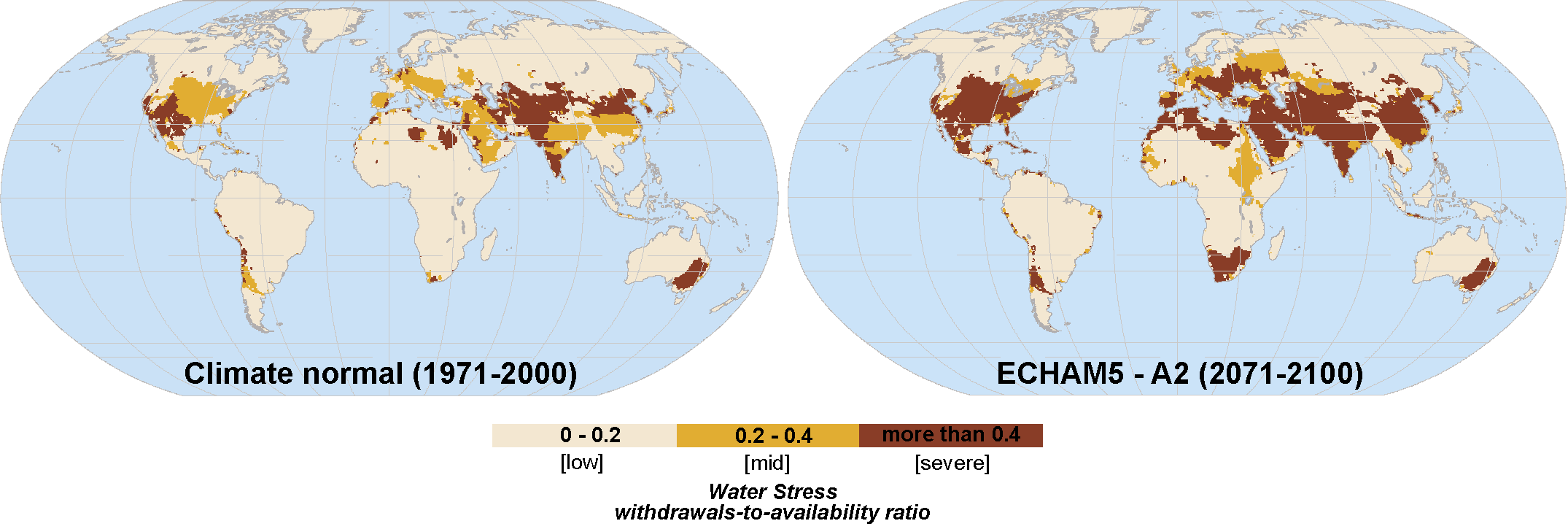
Figure 1: Water stress, calculated as the ratio between water withdrawals and availability, for the late 20th and 21st centuries (see Flörke and Eisner 2011). |
Climate models continue to suggest decreases of rainfall in the semi-arid regions of the world, such as the Mediterranean region, southern USA and Central America, southern Australia and southern Africa. When translated into river flows and available water we predict increasing water scarcity in these regions but also in China, India and the Middle East, where populations and water consumption are rising fast (Fig. 1).
There is considerable variation in the both the global hydrology and climate models (Haddeland et al. 2011). Also regional analyses require the incorporation of many additional processes, such as irrigation and groundwater (and the interactions between them). At present the best approach seems to be to use an ensemble of available hydrological models in tandem with the ensemble of climate models used by the Intergovernmental Panel on Climate Change.
There has been considerable progress on quantifying the global and regional terrestrial water balance in recent years. Considerable uncertainties, however, remain particularly at the regional scale where in situ data on rainfall and runoff are limited. Satellite products and modeling can to an extent fill these gaps, but there remains a need to maintain surface based networks and the free flow of data.
selected references
Full reference list online under: http://pastglobalchanges.org/products/newsletters/ref2012_1.pdf
Flörke M and Eisner S (2011) The development of global spatially detailed estimates of sectorial water requirements, past, present and future. WATCH Technical report number 46
Haddeland I et al. (2011) Journal of Hydrometeorology 12(5) 869-884
Edward R. Cook
Lamont-Doherty Earth Observatory, Columbia University, Palisades, USA; drdendroldeo.columbia.edu
 |
|
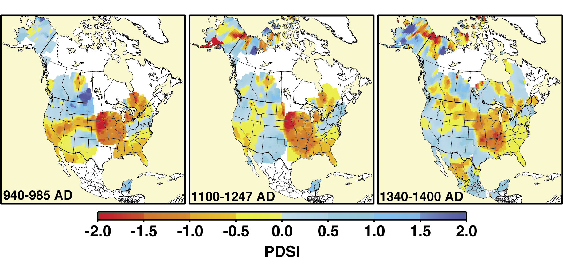
Figure 1: Examples of three megadroughts reconstructed from tree rings that hit the central Mississippi Valley of the United States during early, middle, and late medieval times. See Cook et al. (2010b) for details. |
Climate model projections of future hydroclimatic change associated with increasing atmospheric greenhouse gas concentrations are sobering and, depending on where you live, very alarming. For example, southwestern North America is projected to enter into a long-term drying trend in the sub-tropics to mid-latitudes, and this trend in increasing aridity may have already begun (Seager et al. 2007a). Thus, the unprecedented 2011 Texan drought (www.ncdc.noaa.gov/sotc/drought/2011/8) is an example of what might happen with increasing frequency and duration in the future. Independent of whether or not model projected radiatively forced drying is actually happening now, there is abundant paleoclimate evidence for the occurrence of past “megadroughts” in North America (Stine 1994; Woodhouse and Overpeck 1998; Cook et al. 2004, 2007; Stahle et al. 2011), Asia (Buckley et al. 2010; Cook et al. 2010a), and Europe (Helama et al. 2009; Büntgen et al. 2011) that dwarf any periods of drought seen in instrumental climate records over the past century. The seminal property of megadroughts that differentiates them from even the most severe droughts observed today is duration (Herweijer et al. 2007), with the former often lasting several decades to a century or more compared to just a few years to a decade or so for the latter. Figure 1 shows three such megadroughts reconstructed from tree rings (Cook et al. 2010b) that hit the Mississippi Valley of the United States during early, middle, and late medieval times. These megadroughts lasted 46, 148, and 61 years, respectively, and are ominously located in the American “bread basket” where similar droughts in the future would have catastrophic consequences on agricultural production. This also means that water resources planning and infrastructure design based on observed hydroclimatic data are unlikely to be resilient enough to handle the possible return of megadroughts that we now know have happened in the past.
The cause of past megadroughts is still not fully understood, but persistent patterns of cold La Niña-like sea surface temperatures in the eastern equatorial Pacific ENSO region have been strongly implicated in North America (Herweijer et al. 2006; Seager et al. 2007b; Graham et al. 2007), along with the possible influence of the Atlantic Ocean there as well (Feng et al. 2008). Perhaps more importantly, the paleoclimate record indicates that megadroughts occurred more often during an earlier period of generally above average temperatures called the Medieval Warm Period (MWP), approximately 700 to 1,200 years ago. It is not important to know whether or not the MWP was as warm as today (cf. Crowley and Lowery 2000; Bradley et al. 2003; Mann et al. 2009; Ljungqvist et al. 2011). Rather, the paleoclimate record of past megadroughts simply tells us that 1) they are a natural part of the climate system with no need for anthropogenic greenhouse gas forcing to ignite and sustain them, and 2) rather ominously they appear to “like” warmer climates such as that which occurred during the MWP. Given the climate model projections of future drying and the high likelihood that global warming will continue throughout the 21st century (IPCC 2007), we may therefore be entering into a new era of megadroughts with potentially catastrophic consequences to water supplies needed for human consumption, agriculture, energy production, and for maintaining the aquatic environment. The degree to which any future megadroughts caused by human-induced global warming will resemble those in the past is unclear because the climate forcings operating today are different from the past. Regardless, the stage appears to be set now for some possibly radical future changes in hydroclimatic variability if the past is any guide.
selected references
Full reference list online under: http://pastglobalchanges.org/products/newsletters/ref2012_1.pdf
Bradley R S, Hughes MK and Diaz HF (2003) Science 302: 404-405
Cook ER, Seager R, Cane MA and Stahle DW (2007) Earth Science Reviews 81: 93-134
Cook ER et al. (2010a) Science 328(5977): 486-489
IPCC (2007) Climate Change 2007: The Physical Science Basis. Solomon S et al. (Eds) Cambridge University Press, 996 pp
Sandra Lavorel
Laboratoire d’Écologie Alpine, CNRS, Université Joseph Fourier, Grenobles, France; Sandra.Lavorelujf-grenoble.fr
 |
|
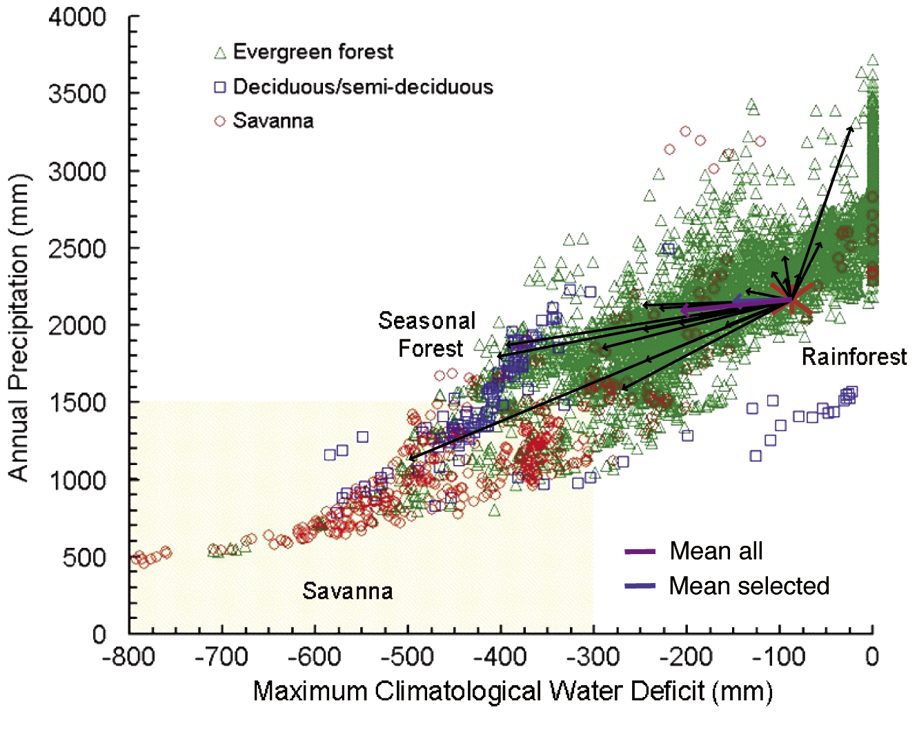
Figure 1: Type of vegetation in relation to rainfall in the Amazon region. The overlaid arrows show the trajectories of change as simulated by the 19 general circulation models used in the IPCC AR4 forced to start from the averaged observed climate over the period 1970-1999 AD (red star). The tips of the arrows represent the simulated late 21st-century (2070-2099 AD) rainfall regime. The purple arrow shows the mean of all model trajectories and the blue arrow the mean of all models that simulate the late 20th century adequately. Figure modified from Mahli et al. (2009). |
Ecosystem services, the benefits humans derive from the biodiversity and functioning of ecosystems, provide a direct link between society and the modifications to the biosphere in response to climate change. Examples of services include crop and forest products, climate regulation through carbon fixation, crop and wild plant pollination by native insects, and recreational, esthetic or religious values. In some regions, the prospect of a warming climate portends a change for the positive: it will allow the production of new crops including cereals or wines of high market value, increased production of some forest species or more enjoyable weather for tourism. However, such positive changes and associated opportunities are not the rule: abrupt changes in ecosystem services associated with climate change are already being observed, and many more are expected (Mooney et al. 2009).
The destruction of entire ecosystems is the most extreme manifestation of the effect of a changing climate. Consider the case of coral reefs, which serve as nurseries for many fish species. As water temperatures rise, bleaching of reefs deprives local populations of important resources from fishing (Hoegh-Guldberg et al. 2007). Coral reef loss also exposes local populations to increased risks from storm damage. Furthermore, income from tourism is lost and thereby an important incentive for sustainable coastal management. Finally, we lose an irreplaceable cultural asset at a global level.
Another example comes from the southwestern United States. A regional-scale tree die-off in semiarid woodlands following the drought in the year 2000 has been referred to as an ecosystem crash (Breshears et al. 2011). The death of trees cascaded to widespread mortality of other species, from pinyon to juniper woodlands. This abrupt event likely altered most ecosystem services fundamentally, with both positive and negative effects. There were short-term effects on grass availability for ranchers (positive), culturally important products such as pinyon nuts (negative) and overall cultural landscape value (negative). Longer-term effects concerned soil erosion and regional climate through changed albedo.
At the planetary scale, although model projections remain conflicting, the shrinking of the Amazon rainforest due to climate change and ensuing land-atmosphere feedbacks has been shown to have potential dramatic consequences for global climate (Mahli et al. 2009). Seemingly less striking changes can entail equally dramatic consequences. Because biotas are the providers of ecosystem services, shifts in the distribution of functionally important species have the potential to disrupt ecosystem services. The distributions of plants and their pollinators can be modified independently from each other, either because of different response speeds or because they are driven by different climatic variables.
Even before the changes in distributions, the subtle matching in phenologies between plants and pollinators is lost and so is the service of pollination, with costly consequences for food production and for culturally important rare species. Conversely, climate change is a golden opportunity for some pest species when their phenology or their distribution synchronizes with those of host plants. Several such cases have already been observed in forest species, such as the altitudinal expansion of the common mistletoe and of the pine processionary moth in the European Alps.
A spectacular case is that of the mountain pine beetle in North America (Kurz et al. 2008). With warming climate this species has been expanding northwards, affecting millions of hectares of coniferous forest. Compounded with increasing fire risk during warmer and drier summers, highly flammable beetle damaged forests have contributed to dramatic increase in burned areas, with considerable effects on regional carbon budgets (expected average emissions for western Canada: 36 g C m-2 yr-1) and potential positive climate feedbacks. The same type of dynamics applies to invasive species, when the climate-driven expansion of exotics such as C4 grasses into shrubby ecosystems (Australia, Cape Region of South Africa) profoundly modifies long-term fire regimes.
Such abrupt changes in ecosystem services are serious challenges to adaptive capacity. Learning from past events, detecting early warning signals and fostering resilience of socio-ecosystems will be essential.
selected references
Full reference list online under: http://pastglobalchanges.org/products/newsletters/ref2012_1.pdf
Breshears DD, Lopez-Hoffman L and Graumlich LJ (2011) Ambio 40: 256-263
Hoegh-Guldberg O et al. (2007) Science 318(5857): 1737-1742
Kurz WA et al. (2008) Nature 452: 987-990
Mahli Y et al. (2009) PNAS 106(49): 20610-20615
Mooney H et al. (2009) Current Opinion in Environmental Sustainability 1: 46-54
Stephen T. Jackson
Department of Botany and Program in Ecology, University of Wyoming, Laramie, USA; Jacksonuwyo.edu
Although “ecosystem services” is a relatively new term, the concept has a long history. For example, the 1895 New York State Constitution designated the Adirondack Forest Preserve to be “forever wild” in order to maintain water quality and supply in the Hudson River watershed. Ancient societies utilized such ecological goods as fuels, fibers, and foods deriving from natural or lightly managed ecosystems, and many came to recognize the ecological services provided by vegetated watersheds and floodplains. Such recognition often came the hard way, just as it does for modern societies.
Studies of the past play important roles in assessing risks and vulnerabilities for ecosystem services in two ways: by providing records of interactions among environmental change, ecosystem services, and societal activities, and by showing how ecosystem properties that underlie ecosystem services have been affected by climatic changes. Because human activities have affected ecosystems for centuries to millennia, it is particularly important to establish baselines for ecosystem properties and services, and to determine how those baselines have already been altered by humans. Teams of marine biologists and paleobiologists have documented history of human impacts on North American fisheries (Jackson et al. 2001; Jackson 2001). Although Native Americans harvested fish and shellfish, often intensively, estuarine ecosystems were little affected. However, introduction of European technologies led to rapid size decline of fish at the top of the food chain, and intensive oyster harvesting resulted in estuarine eutrophication. Both trends accelerated with industrial fishing of the 20th century, with multiple consequences for ecosystem goods and services.
In another example, alpine lake sediments in the western United States record a five-fold increase in dust deposition concurrent with intensive cattle and sheep grazing in the 19th century (Neff et al. 2008). Modeling studies reveal that the dust emissions, caused by breakup of soil crust and reduction of vegetation cover at low elevations, were sufficient to reduce snow albedo, shortening high-elevation snow-cover by several weeks and altering seasonal and total stream discharge (Painter et al. 2010). The sediment studies also show that federal grazing regulations introduced in the 1930s had mitigating effects on dust deposition (Neff et al. 2008).
_LvG_opt.png) |
|
Figure 1: Geohistorical records of temporal changes in ecosystem properties and services. This 3000-year composite record of regional ecosystem attributes (land cover, erosion, flood intensity) inferred from sediments of Lake Erhai and monsoon intensity inferred from a speleothem shows ecosystem responses to changes in human population, cultural practices, and climate. The five green bands show primary periods of human effects on the regional environment (left to right): Bronze-Age culture, Han irrigated period, Nanzhao Kingdom, Dali Kingdom, and late Ming/early Qing environmental crisis. (From Dearing 2008). |
These studies focus on impacts during the historical period, but ancient societies also provide object lessons on interactions among cultural practices, climate change, and ecosystem services (Costanza et al. 2007; Büntgen et al. 2011). Sediments from Lake Erhai in southwestern China show vividly how a succession of late Holocene cultures influenced land-cover, soil erosion, and flooding (Fig. 1), culminating in a peak of land clearance and soil erosion in the 17th and 18th centuries (Dearing 2008; Dearing et al. 2008). Consequences of land-use practices may have interacted with increasing monsoon intensity, leading to a well-documented environmental crisis that began to abate only in the 20th century.
Studies of environmental and ecological changes, even without direct links to cultural practices or consequences, play important roles in assessing ecosystem services. Ecosystem services ultimately derive from structural, functional, and compositional properties of ecosystems, and understanding how those properties have responded to past climate changes can provide insight into vulnerability of ecosystem services to ongoing and future climate change (Williams et al. 2004; Jackson 2006; Jackson et al. 2009). North American mid-continental droughts in the Holocene provide a series of case studies. Most recently, multidecadal droughts associated with the Medieval Climate Anomaly led to widespread changes in fire regime and vegetation composition in the central and western Great Lakes region (Shuman et al. 2009; Booth et al. 2012). In the mid-Holocene, a severe and persistent drought (ca. 4200-4000 a BP) resulted in forest disturbance and compositional change in the western Great Lakes as well as dune mobilization in the Upper Mississippi Valley (Booth et al. 2005). In the early Holocene, the mid-continent experienced a gradual, time-transgressive drying, punctuated by a rapid, region-wide drying associated with final collapse of the Laurentide ice sheet. Ecosystem responses show both gradual and time-transgressive trends and a step-change associated with the rapid event (Williams et al. 2009, 2010). Timing varied widely among individual sites, suggesting different thresholds and sensitivities of local systems. All these case studies indicate that ecosystem properties, and ultimately ecosystem services, are vulnerable to climatic change, whether transient or persistent, and that sensitivity varies substantially among ecosystems and regions.
selected references
Full reference list online under: http://pastglobalchanges.org/products/newsletters/ref2012_1.pdf
Costanza R, Graumlich LJ and Steffen W (2007) Sustainability or Collapse? An Integrated History and Future of People on Earth, MIT, 520 pp
Dearing JA (2008) The Holocene 18: 117-127
Jackson JBC et al. (2001) Science 293: 629-638
Abrupt changes - To what extent are tipping points a concern in coping with global change? [Present]
Derek Lemoine
Department of Economics, The University of Arizona, Tucson, USA; dlemoineemail.arizona.edu
Tipping points have entered common discourse in a range of applications: the uprisings of the Arab Spring, the narrative of sporting events, the evolution of consumer sectors, the rhythm of political campaigns, the threat of space junk, and the collapse of financial systems. An increasingly frequent application concerns the changing climate (Russill and Nyssa 2009). Some climate tipping points irreversibly change social structures, and the form of this change determines the ultimate effect on climate damages.
Undesirable tipping points involve climate change impacts. First, consider New Orleans or Bangladesh. The infrastructure in these regions are increasingly stressed due to higher sea levels and disappearing wetland buffers. Changing conditions have made them more vulnerable to future storms that could trigger a tipping point for the local culture and economy. Or consider a climate-induced drought that shifts a livestock-based economy to less water-intensive activities. These changes become partially irreversible as economic activity, infrastructure, and communities reorganize under new constraints.
Second, and perhaps more troublingly, climate change might induce large-scale migrations due to higher sea levels, water stress, crop failures, or extreme weather events (de Sherbinin et al. 2011). Shifting populations have triggered massive changes throughout world history, and future migrating populations could trigger internal or external conflicts and bring new challenges of assimilation and adjustment. For example, climate change could enhance water scarcity in South Asia, and recent conflicts in Darfur and other parts of Africa might have been exacerbated by environmental problems.
Other societal tipping points are desirable. First, a breakthrough in low-carbon technology might be necessary to change the dynamics of the energy system (Hoffert et al. 2002). If solar cells or batteries become cheap enough, electrical and transportation systems could begin shifting to less carbon-intensive structures even without a direct policy spur. Second, enacting a greenhouse gas emission policy should create constituencies for further policy. Ambitious policies currently lack clearly defined winners to lobby for their enactment, but moderate policies could develop this constituency by coining valuable property rights in tradable permits or by nurturing low-carbon industries. Third, on the international level, a climate coalition that includes enough countries might be able to raise remaining countries’ cost of holding out (Barrett 2003).
 |
|
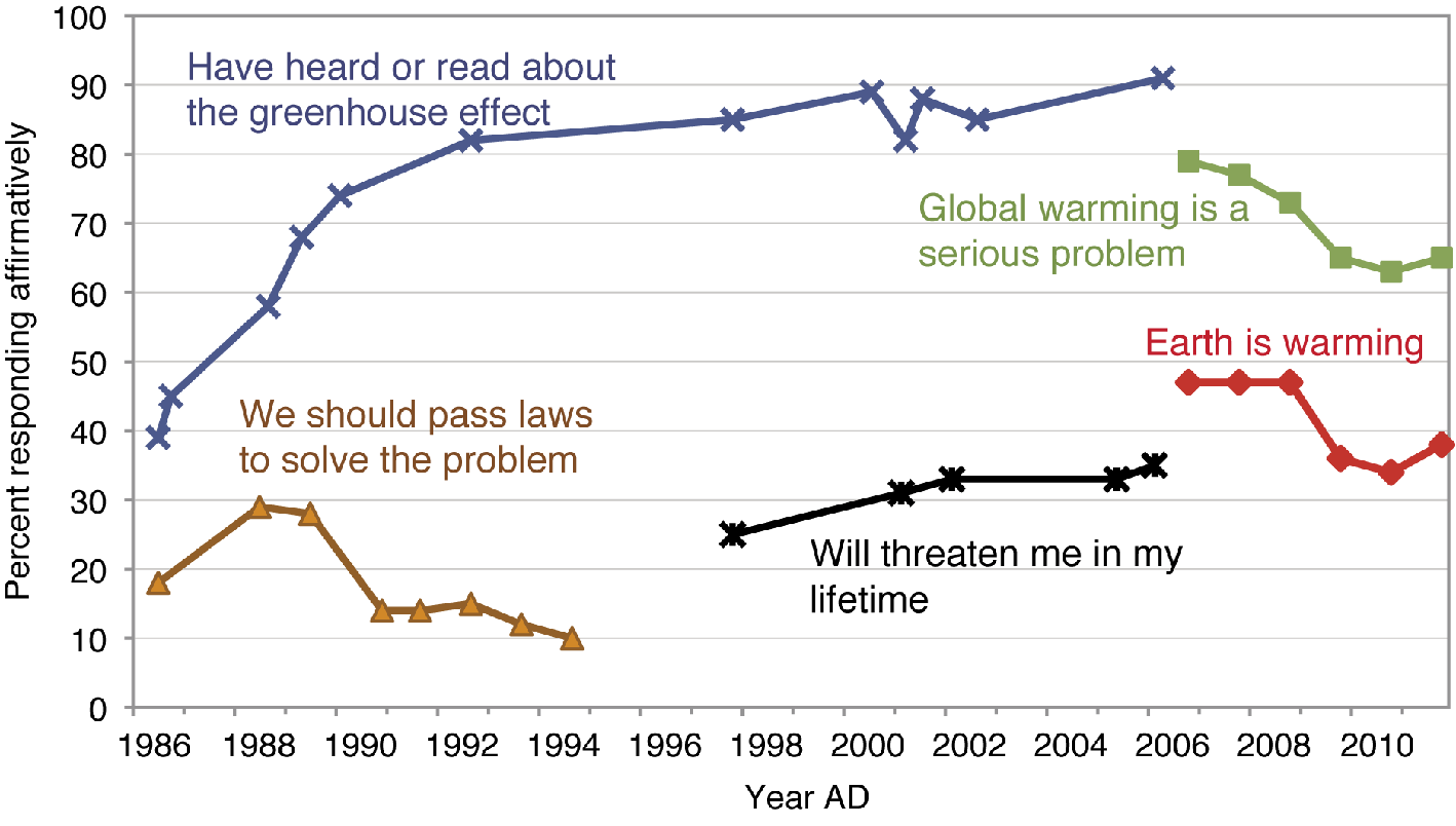
Figure 1: The response of the U.S. public to surveys’ questions about global climate change (Pew Research Center for the People & the Press; Nisbet and Myers 2007). |
Finally, we may still reach a further tipping point in climate awareness (see figure 1). Drawing on examples ranging from the diffusion of rumors to trends in smoking, some argue that social networks allow beliefs and behaviors to spread quickly once they reach a critical mass (Gladwell 2000). Incurring undesirable tipping points could raise public concern about the climate to such a threshold. Similar to how the first exposure to the horror of nuclear weapons has so far kept the world from further nuclear warfare, reaching the first undesirable climate tipping point may end up making future tipping points less likely by spurring preventive action.
From economic analysis of tipping points in the physical climate system, we have shown that the best policy response to a tipping possibility depends on two questions: (1) Can we affect whether a tipping point occurs? (2) If we knew a tipping point were about to occur, would we want to pursue a different policy? The first question captures our ability to prevent or spur a tipping point, while the second captures our desire to hedge against the possibility that it occurs. Because the undesirable tipping points depend on our present and future emission decisions, they provide additional incentive to reduce emissions. These undesirable tipping points also increase the payoffs to adaptation policies that reduce society’s exposure to a changing climate. In contrast, desirable tipping points favor policies that make them more likely: funding research into low-carbon technology, pricing carbon sooner rather than later, and building climate awareness. If these desirable tipping points end up spurring significant emission reductions, they might even hold the key to avoiding undesirable ones.
selected references
Full reference list online under: http://pastglobalchanges.org/products/newsletters/ref2012_1.pdf
Barrett S (2003) Environment and Statecraft: The strategy of environmental treaty-making, Oxford University Press, 437 pp
de Sherbinin A et al. (2011) Science 334(6055): 456-457
Gladwell M (2000) The tipping point: How little things can make a big difference, Little Brown, 288 pp
Hoffert M et al. (2002) Science 298(5595): 981-987
Russill C and Nyssa Z (2009) Global Environmental Change 19(3): 336-344
Dorthe Dahl-Jensen
Niels Bohr Institute, University of Copenhagen, Denmark; ddjgfy.ku.dk
 |
|
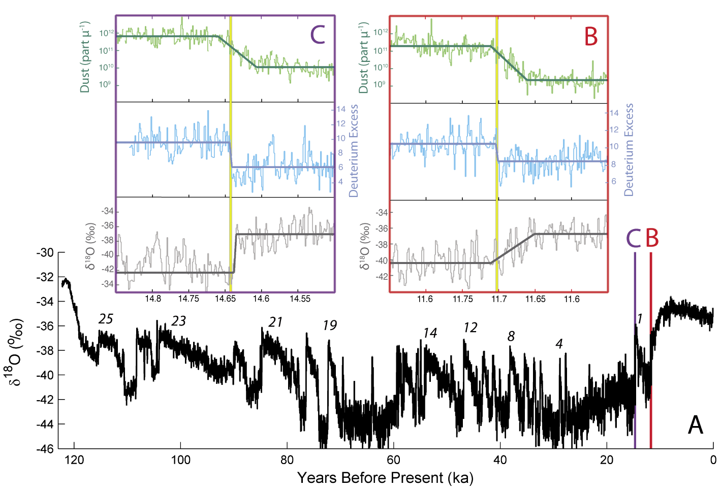
Figure 1: High-resolution records from the Greenland ice core NGRIP. Panel A shows stable water isotopes (δ18O) in 20-year resolution. Numbers mark the most prominent of the 25 Dansgaard-Oeschger events. Panels B and C zoom in on two 300-year intervals during the transition from the last glacial to the Holocene. Shown are records of δ18O, deuterium excess and the unsolvable dust at 1-year resolution. The solid lines highlight the transitions in the records; the vertical yellow lines mark the steps in deuterium excess over just a few years. (Figure based on Steffensen et al. 2008). |
Paleoclimatic records can provide information on the operation of the climate system, including the occurrence of tipping points and the risk of abrupt changes. The deep Greenland and Antarctic ice cores are particularly well suited to study abrupt changes, because they provide a detailed and well-dated record of past climate. Prominent examples of abrupt changes are the 25 Dansgaard-Oeschger (DO) events (NGRIP 2004) that occurred during the last glacial cycle (Fig. 1).
The DO events are characterized by abrupt warming followed by a gradual cooling. The isotopic composition of the nitrogen (N2) in air bubbles trapped in Greenland ice and the stable water isotopes of oxygen (18O) and hydrogen (deuterium, D) of the ice itself show that the abrupt warmings represent surface temperature changes in the order of 10-15°C (Landais et al. 2005). Annually dated ice core sections covering the two most recent DO events reveal the actual rapidity of the changes. Some proxies, like the deuterium excess (d=δD-8*δ18O), changed level over just a few years (Steffensen et al. 2008). The deuterium excess reflects the temperature at the moisture uptake region for the precipitation. Its step-like changes in Greenland ice cores suggest that the atmospheric circulation regime shifted substantially and irreversibly basically from one year to the next (Masson-Delmotte et al. 2005). Following the atmospheric regime shift, temperatures over Greenland warmed more gradually over some decades by 10-15°C, as shown by the δ18O record (Steffensen et al. 2008). These observations prove that the climate system did, and therefore can, tip and reorganize internally within years and cause strong and fast regional temperature changes.
How and why did the abrupt climate changes happen? Studies from all latitudes based on ice cores from Polar Regions, marine sediments, stalagmites, corals and other paleoclimatic archives allow us to piece together a broader picture of the DO events and to deduce a sequence of causes and effects. During the cold phases preceding the abrupt warmings, vast volumes of ice were discharged into the ocean from the large glacial ice sheets including the North American Laurentide ice sheet, causing sea level to rise by several tens of meters (Siddall et al. 2003). The overturning circulation and associated northward heat transport in the Atlantic slowed down. This warmed the South and cooled the northern polar region further and may have resulted in a southward shift of the Intertropical Convergence Zone (ITCZ; Partin et al. 2007).
What caused the abrupt warmings? This is less well understood and requires investigation of the (very sparse) near-annually dated records. The studies from the Greenland ice cores suggest that the sudden rearrangement of the northern atmospheric circulation might have been initiated by a sudden shift of the ITCZ in the low latitudes. A sudden decrease of the dust concentration in the ice indicates that the wetness of the source area for the dust (related to the position of the ITCZ) had shifted (Steffensen et al. 2008). Perhaps the warming of the south finally pushed the ITCZ north again?
Can such tipping points of temperature and sea level change happen in the coming decades and centuries? The DO events during the last glacial seemed to be initiated by surges from big glacial ice sheets. Such large Ice sheets are not present nowadays, but other triggers that could cause the system to tip are plausible. Increased precipitation and melting of ice sheets and glaciers could increase the fresh water supply to the Arctic and the North Atlantic Ocean and alter the intensity of the ocean circulation. This would tip the energy distribution between the North and South in a similar way as happened during the glacial DO events. Rapid mass loss of the West Antarctic Ice Sheet, of which major parts lie more than 1 km below the present sea level, could cause an abrupt sea level rise of several meters.
State-of-the-art simulations with complex Earth System models do not project abrupt climate changes for this century. However, based on our understanding of the past DO events we conclude that abrupt changes of temperature and sea level cannot be ruled out entirely for our future world.
selected references
Full reference list online under: http://pastglobalchanges.org/products/newsletters/ref2012_1.pdf
Partin JW et al. (2007) Nature 449: 452-455
Landais AA, Jouzel J, Masson-Delmotte V and Caillon N (2005) Comptes Rendus Geosciences 337: 947-956
Masson-Delmotte V et al. (2005) Science 309: 118-121
Heinz Wanner1,2 and Stefan Brönnimann1,2
The two main millennial-scale Holocene climate patterns or submodes are also significant at the multidecadal to century-scale level.
Large-scale climate patterns and modes are important instruments to characterize prevalent teleconnections and their related processes. Their correlation with forcing factors constitutes an important element of climate diagnostics. The increasing number of data and modeling studies referring to Holocene climate provokes the question whether or not global patterns or modes predominated.
The millennial-scale pattern
 |
|
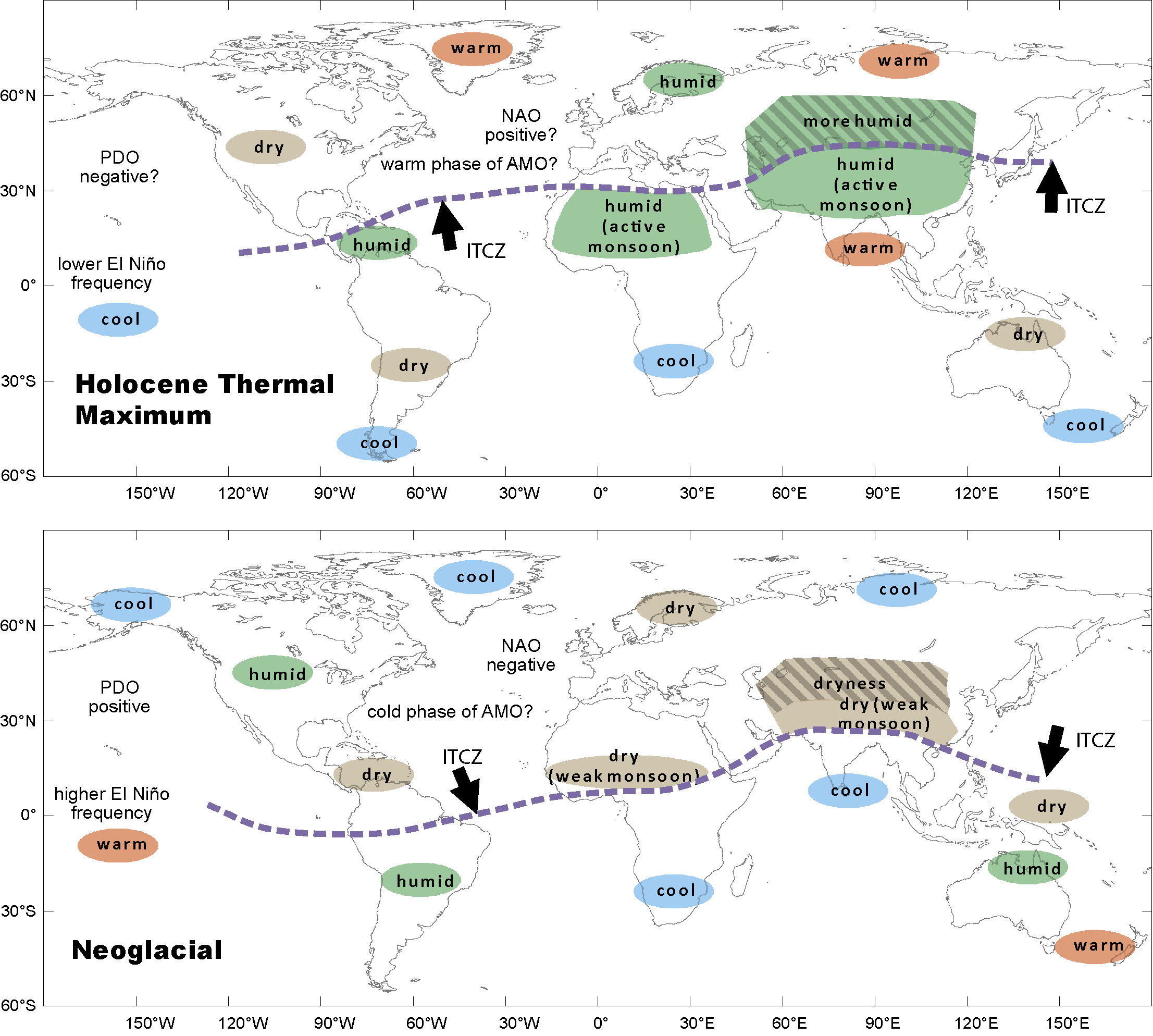
Figure 1: Climate patterns of the Holocene Thermal Maximum (~7-4.5 ka BP; Ljungqvist 2011), and the Neoglacial, which started around 4.2 ka BP and ended with the modern industrialization in the 19th century. Both Figures were outlined based on existing Holocene proxy time series (Wanner et al. 2011). |
The Holocene spans the time period of the last 11.7 ka. During the first 5 ka a reorganization of the hydrographic system due to the melt of the large ice sheets took place (Carlson et al. 2008; Renssen et al. 2007). Apart from the recent decades being influenced by anthropogenic forcing climate change during the period of the last 7 ka was dominated by the decreasing solar insolation in the Northern Hemisphere during boreal summer (Berger 1978; Wanner et al. 2008). Due to this redistribution of solar energy the global climate system experienced rearrangements, which are represented in Figure 1a and b for the Holocene Thermal Maximum (HTM) and the so-called Neoglacial (Wanner et al. 2008).
During the HTM the enhanced heating of the Northern Hemisphere during boreal summer led to a warming generating intensified heat lows and a higher activity of the Afro-Asian summer monsoon systems transporting more moisture to the corresponding continental areas. Positive temperature anomalies in the area of the Indo-Pacific Warm Pool (IPWP) and negative ones in the eastern Pacific area predominated (Xu et al. 2010; Marchitto et al. 2010) and, correspondingly, the El Niño frequency was low (Clement et al. 2000; Rein et al. 2005). For the North Atlantic area some studies (e.g. Rimbu et al. 2003) show that positive North Atlantic Oscillation/Arctic Oscillation (NAO/AO) indices dominated during the early Holocene. No information is available for the Atlantic Multidecadal Oscillation (AMO; Schlesinger and Ramankutty 1994). Even more uncertainties exist in the Southern Hemisphere subtropics and midlatitudes.
An almost opposite pattern existed during the Neoglacial (Fig. 1b). The Intertropical Convergence Zone (ITCZ) shifted to a more southerly position, the Afro-Asian summer monsoon systems were less active, and the corresponding continental areas were exposed to an increasing dryness (Gasse et al. 2000; Haug et al. 2001; Wang et al. 2005). A warmer eastern tropical Pacific and a higher El Niño frequency coincided with predominantly neutral or negative NAO/AO indices and likely led to a more humid climate in the Great Plains and southwestern North America.
A multi-decadal to century-scale Holocene mode explaining climate shifts?
In addition to the orbitally driven solar insolation changes the patterns in Figure 1 were also determined by internal variability, which strongly depends on specific physical boundary conditions, such as land-ocean and sea-ice distribution and topography. In concert with the two other natural forcings (solar, volcanic) characteristic temperature and humidity patterns may have occurred, which could be interpreted as climate modes (Stephenson et al. 2004). One possible way to study long-term global climate variability and change is to investigate the dynamical modes with an annular structure on both hemispheres, expressed by the indices describing the strength of the Westerlies, namely the Antarctic Oscillation (AAO; Thompson and Wallace 2000) and the AO/NAO (Hurrell et al. 2003). The focus of the maps on Figures 1a and b is more directed towards the dynamics in the Atlantic and Pacific areas. The most important mode is located in the Pacific, the area with the highest sea surface temperatures. Its orientation is mostly zonal, and it encompasses the IPWP and the ENSO system, including its connections with the Indian/East Asian monsoon as well as with the Pacific North American Pattern and the Pacific Decadal Oscillation. The orientation of the second mode (NAO/AMO) is rather meridional, including the Atlantic Ocean with the Arctic sea ice and the adjacent continental areas.
How far are ENSO and NAO coupled, and which processes determine the dominating patterns in Figure 1? A first option is to investigate whether or not the two modes are correlated and interact in a systematic manner on short time scales, and then extend the analysis to long time scales. Recent studies (Brönnimann 2007) suggest that a coupling exists, and that it most likely operates through an alteration of the flow over the Pacific-North American-Atlantic sector. However, the coupling is statistically weak and has not been addressed for longer time scales.
A second option is to study the influence of the two major non-orbital natural forcing factors (Shindell et al. 2003): solar and volcanic activity. In case of large tropical volcanic eruptions (Robock and Mao 1995; Fischer et al. 2006) the lower stratosphere is heated more over the tropical regions than near the poles, which accelerates the wintertime polar vortex. Through downward propagation, this can affect the circulation near the ground. Therefore, despite an overall annual mean global surface cooling, the strengthening of the Westerlies (with positive NAO indices) causes higher winter temperatures mainly along the west coasts of the major continents. So-called Grand Solar Minima (GSM; Steinhilber et al. 2009) cause a major cooling especially in the large continental areas of the Northern Hemisphere. Due to their inertia the oceans show a delayed SST response, and negative AO/NAO indices predominate (Shindell et al. 2003; Mann et al. 2009). Whether or not the two forcings affect global climate via altering ENSO is debated (Adams et al. 2003; Mann et al. 2005; Meehl et al. 2009). At least during the early Holocene periods of low solar activity corresponded with El-Niño-like (warm) conditions, weak Asian monsoons and low SSTs in the North Atlantic (Marchitto et al. 2010).
A third option is to study the frequency and the strength of important modes during periods with predominating warm or cold temperature anomalies. On the basis of petrologic tracers in the North Atlantic, Bond et al. (1997 and 2001) postulated a “1500 year” cycle that is supposed to have persisted throughout the Holocene. These cycles were thought to be the Holocene equivalents of the Pleistocene Dansgaard-Oeschger cycles (Alley 2005). Several authors (e.g. Hong et al. 2003; Gupta et al. 2005; Wang et al. 2005) speculated that a link existed between the weak Indian/Asian summer monsoon and the cool North Atlantic climate, which was possibly triggered by solar influence. Recent studies show that different dynamical processes were likely responsible for the existence of the Bond cycles (Wanner and Bütikofer 2009). Prior to the modern warm period with anthropogenic forcing, the last 2 ka included two warmer (Roman Warm Period RWP, Medieval Climate Anomaly MCA) and two cooler periods (Migration Period Cooling MPC, Little Ice Age LIA). It is still debated whether or not those phenomena were global. The solar activity was obviously higher and the volcanic forcing weaker during the RWP and the MCA (Steinhilber et al. 2009), and a shift from positive to negative NAO indices might have occurred during the MCA-LIA transition (Trouet et al. 2009; Mann et al. 2009). Similar to the pattern in Figure 1a multidecadal droughts occurred in southwestern North America during the RWP (Routson et al. 2011) and during the MCA (Seager et al. 2007), possibly linked with La Niña-like conditions and positive NAO indices.
Interestingly, a rapid shift to more humid conditions was observed during the LIA, mainly in the tropics (Wanner and Ritz 2011). Gagan et al. (2004) postulate that the tropical Pacific played a role as a source region of water vapor during the expansion of the LIA glaciers. The LIA was characterized by a coincidence of large explosive volcanic events and strong solar minima (Breitenmoser et al. 2011). While during the MPC a remarkable GSM took place around AD 650 (Steinhilber et al. 2009) the RWP shows neither strong volcanic events nor a GSM. On the other hand the oscillations in the early Holocene (Marchitto et al. 2010) as well as the MCA-LIA transition were exposed to stronger forcings and show patterns similar to the millennial scale ones in Figure 1a and b.
We could therefore pose the question whether or not these patterns represent the features of a characteristic multi-decadal to century scale climate mode. If the two patterns in Figure 1 represent two specific submodes of Holocene climate, the question can be asked whether one of them could dominate in the future under the influence of anthropogenic climate change.
affiliations
1Institute of Geography, University of Bern, Switzerland; wanneroeschger.unibe.ch
2Oeschger Centre for Climate Change Research, University of Bern, Switzerland
selected references
Full reference list online under: http://pastglobalchanges.org/products/newsletters/ref2012_1.pdf
Bond G et al. (2001) Science 278: 1257-1266
Brönnimann S (2007) Reviews of Geophysics 45, doi: 10.1029/2006RG000199
Marchitto TM et al. (2010) Science 330: 1378-1381
Wanner H et al. (2008) Quaternary Science Reviews 27: 1791-1828