PAGES Magazine articles
Madelyn J. Mette![]() 1, T. Trofimova
1, T. Trofimova![]() 2, S.J. Alexandroff
2, S.J. Alexandroff![]() 3 and E. Tray
3 and E. Tray![]() 4
4
Horizon scanning is an exercise which aims to collaboratively identify research priorities within a field. As exemplified by recent work led by members of the PAGES Early-Career Network in the field of sclerochronology, additional benefits include gained experience in collaboration, networking, and knowledge development.
Defining top research priorities within a discipline is a common pursuit toward advancing the state of the art. An increasingly applied strategy, termed "horizon scanning", relies on community-based input and collaboration through surveys and rating systems to develop a combined perspective on important emerging topics and/or persistent challenges in the field (Sutherland et al. 2011). The concepts are then presented as research questions to be addressed within continuing and future work, providing a kind of roadmap for development of the field (for recent examples see Patiño et al. 2017; Sutherland et al. 2020).
 |
|
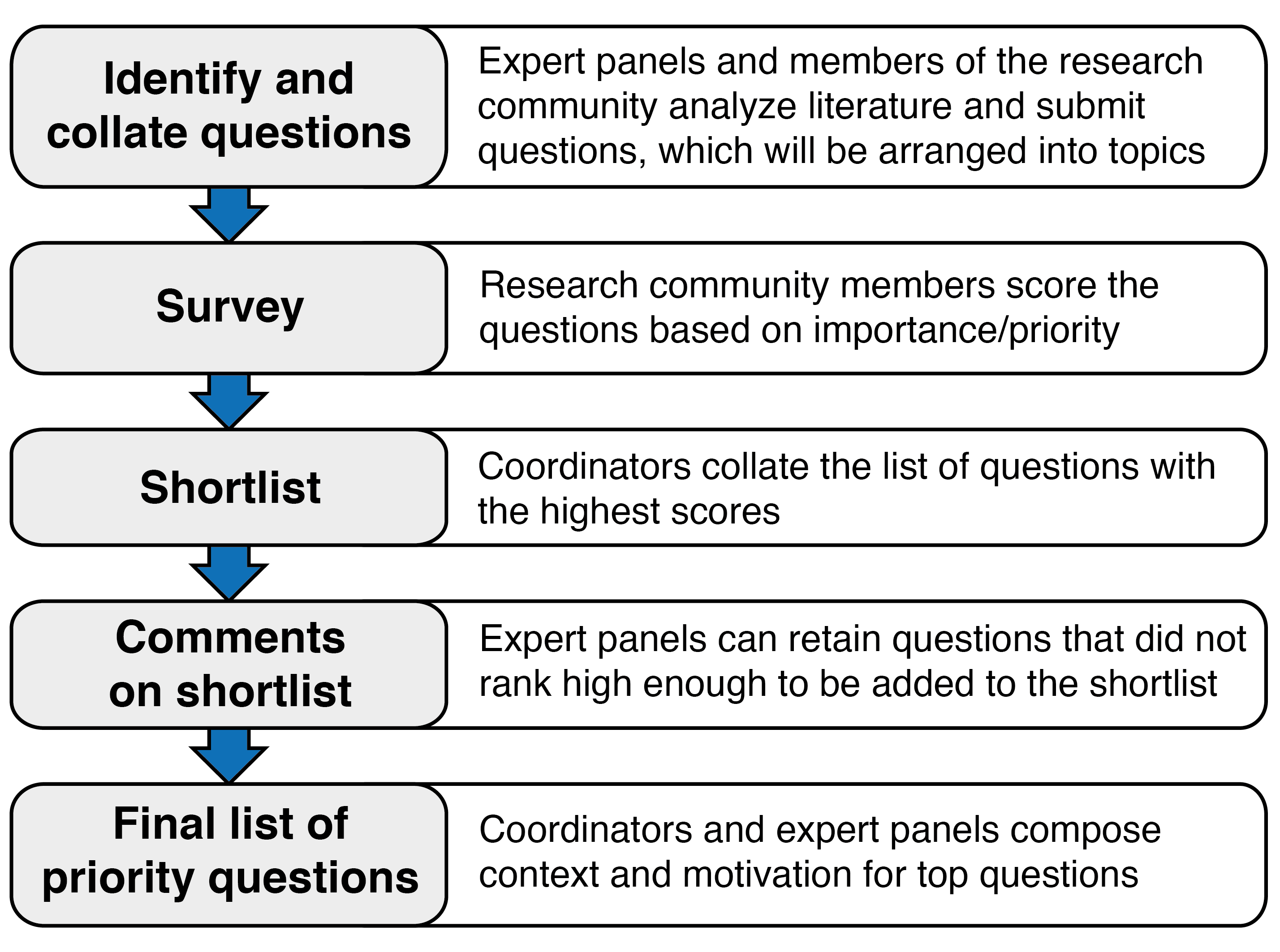
Figure 1: A brief overview of the horizon-scanning process in sclerochronology. |
Following this objective, four members of the PAGES Early-Career Network (authors of this article; PAGES ECN; pastglobalchanges.org/ecn), recently led a horizon-scanning exercise for the field of sclerochronology. This field encompasses the study of physical and chemical variations in the accretionary hard tissues of organisms, and the temporal context in which they formed. Physical and geochemical proxies from coral, bivalve, and otolith archives, for example, contribute to research questions across ecology, paleoclimatology, archaeology, and other fields. Sclerochronology has experienced significant growth over the past decade, with new methods and applications continually being explored. Because of this, we realized the need and an opportunity to formulate research priorities within our field.
Published as part of a special issue after the 5th International Sclerochronology Conference in Split, Croatia (ISC; June 2019), a manuscript by Trofimova et al. (2020) represents the first peer-reviewed scientific product by the PAGES ECN. The manuscript was strengthened by the significant involvement of 23 additional experts (and coauthors) in sclerochronology. The work can serve as a long-standing resource to be reassessed as the field develops. Completion of the project gives us the opportunity to reflect on the process and its impact on those involved. In this article, we provide a brief description of our process and scientific findings followed by discussion of some of the strategies we used and lessons learned in our approach to collaboration. We suggest that such horizon-scanning projects can provide huge benefits to early-career researchers, especially by giving them increased visibility, allowing them to develop a better understanding of the subject area, and providing them with invaluable experience in international collaboration.
 |
|
Figure 2: Organization of categories and topics encompassing the horizon-scanning project in sclerochronology, spanning development across foundations and applications of the field. Additional questions retained by expert panels (Cutting-edge) were also presented. |
Overall process
The sclerochronology horizon-scanning exercise involved soliciting "high priority" research questions from the sclerochronology community, compiling and categorizing the questions, returning the list to the community in the form of a priority-ranking survey, and, ultimately, presenting the top 50 priority research questions alongside brief descriptions of their context and motivation (Fig. 1). The questions were divided into two broad categories: foundations and applications (Fig. 2). Foundations in sclerochronology include questions addressing knowledge gaps in our understanding of sclerochronological archives. This category was further divided into six subtopics. Applications encompass the use of sclerochronological techniques to address long-standing research questions in other fields. This category was divided into three subtopics. An extra category, Cutting-edge sclerochronology, comprised questions that expert coauthors deemed significant or uniquely important even though the community had not ranked them within the top 50.
Results
While the field of sclerochronology has experienced rapid growth over the past few decades, the top priority questions ranked by the community reveal that there is still significant advancement to be made in building upon our foundational knowledge (i.e. the underlying basis for proxy application). For example, an emergent theme from the Foundations section was the need for a better understanding of the mechanisms behind biological control over biomineralization. Top questions also emphasized the establishment and widespread use of common standards for data management and analysis as an important strategy to enable future work. The large number of questions that were focused on applications, however, suggests the field is developed enough to provide new insights into important topics across the natural and social sciences. Top questions highlighted the precise dating and high resolution (at least annual) attainable from many sclerochronological archives as key advantages to solving long-standing questions in climate science and ecology, in particular. The entire list of highest-ranked questions recognizes the breadth of opportunity within the field of sclerochronology (Foundations and Applications), while also acknowledging novel applications that may have been overlooked in the ranking process (Cutting-edge sclerochronology).
Strategies and lessons learned
The triennial ISC provided a venue to discuss our idea with senior colleagues, gain commitment from collaborators, and establish processes moving forward. Project leaders and invited experts shared and debated feedback on our proposed goals and approach. After the conference, the wider sclerochronology community was invited, via email list servers and social media, to submit research questions they deemed important. With 202 initial submissions, deciding how much editorial liberty we should exercise to arrive at a consistent format and use of terminology was a great challenge. Most suggestions required some reformatting in order to be presented on an equal playing field while still preserving their original intent. Providing more clear and strict guidelines during the question submission phase may have alleviated this challenge to some extent.
During our discussions with experts, alternative visions for the article were shared, including the suggestion to present only a handful of broad research "themes" for future work. While we found these suggestions valuable, we were committed to following a traditional horizon-scanning model as exemplified in other fields (e.g. Seddon et al. 2014; Sutherland et al. 2020) as the first such exercise to be performed in sclerochronology. The final list of questions provides ideas for future work and can be pursued as either part or the whole of individual projects. While research groups independently defining their own research agendas can certainly lead to innovation and progress, a unified research agenda provides an opportunity to cooperatively and more rapidly move the field forward (Sutherland and Woodruff 2009). Furthermore, presenting focused research questions to the community may encourage multiple, reproducible studies on the same subjects, which is essential for reaching scientific consensus. We ultimately received strong and continuous support in this effort throughout the project. Indeed, because we as early-career researchers will inherit the future of the field, we were granted the freedom to follow our vision for contributing to that future.
The broad call to the scientific community resulted in a bias toward some of the most commonly studied archives (bivalves, otoliths), well-represented regions (North Atlantic, Europe), and prevalent research applications (climate science, ecology) presented at the ISC conferences. While an effort was made to properly acknowledge and overcome this bias (see Trofimova et al. 2020 for further discussion), we believe that seeking out the involvement of research groups, more directly and from different fields and regions, could help improve representation across the diversity of sclerochronology, thus providing a more valuable result overall.
We resolved the challenges discussed above through successful international collaboration. Because it was unfeasible to hold virtual meetings with all or even most coauthors, communication to the project team occurred through email and file sharing. The lead authors were primarily responsible for managing questions, discussions, and feedback on two to four subtopics each, followed by review or input on all other subtopics. The coauthors were assigned to expert panels that aligned with their research expertise and tasked with providing feedback on those subtopics. All coauthors had access to one shared document, stored in a cloud, and were given clear instructions on how to use online tools for adding content or providing feedback. This strategy was critical in keeping all authors involved and updated.
Key insights
The collaborative nature of horizon scanning offers an approach which allows early-career researchers, in particular, to significantly contribute to the future of a field. A meaningful byproduct of the exercise was increased visibility, collaborative experience, and knowledge development for those involved. After completion of our horizon-scanning project in sclerochronology, we all felt more equipped to approach multiple subtopics within our field with confidence, having had the opportunity to lead in-depth scientific discussions and help find a consensus among a community of experts. Few other research or training activities could have provided such a comprehensive and rigorous experience. While our project occurred before the COVID-19 pandemic, we recognize that horizon-scanning initiatives may represent prime opportunities to perform large collaborations without the requirement of in-person meetings. The PAGES ECN is well equipped to foster such collaborations through horizon-scanning projects, data compilations, review papers, new research projects, and other pursuits that benefit from broad collaboration.
affiliations
1US Geological Survey, St. Petersburg Coastal and Marine Science Center, St. Petersburg, Florida, USA
2NORCE Norwegian Research Centre, Bjerknes Centre for Climate Research, Bergen, Norway
3College of Life and Environmental Sciences, University of Exeter, UK
4Marine and Freshwater Research Centre, Galway-Mayo Institute of Technology, Ireland
contact
Madelyn Mette: mmette usgs.gov
references
Patiño J et al. (2017) J Biogeogr 44: 963-983
Seddon A et al. (2014) J Ecol 102: 256-267
Sutherland W, Woodruff H (2009) Trends Ecol Evol 24: 537-527
Sutherland W et al. (2011) Methods Ecol Evol 2: 238-247
Nikita Kaushal![]() 1, Y. Kulkarni
1, Y. Kulkarni![]() 2, P. Srivastava
2, P. Srivastava![]() 3, S. Rawat
3, S. Rawat![]() 4 and S. Managave
4 and S. Managave![]() 5
5
Speleothem, tree-ring, and borehole archives represent the majority of publicly available proxy data from the terrestrial Indian region for investigating local climatic responses to past global circulation changes. Increasing access to data from lake-sediment archives will open new opportunities for climate research in this region.
A case for data
In the last decade, the paleoclimate field has made tremendous progress in the domains of statistical analysis of regional- to continental-scale proxy data (Tardif et al. 2019), numerical modeling (Owen et al. 2018), and data-model comparisons (Comas-Bru et al. 2019) to gain a better understanding of the processes driving climate and to improve future climate predictions. However, these analyses are only possible if data are made available by the initial data generators in supplementary information sections of published articles or in online data repositories. Synthesizing data from these different sources for regional- to continental-scale data analysis then requires further data wrangling, which is estimated to consume 80% of researcher time in some scientific fields (Dasu and Johnson 2003). The NOAA, PANGAEA, and Neotoma repositories and PAGES working groups address this issue by standardizing and, in some cases, synthesizing data. Here, we examine proxy data from the terrestrial Indian region available from the aforementioned sources and suggest the best ways to access data. We show gaps between data that have been measured but are not yet available, which will require an archive-specific, community-based effort. We highlight data that are available and should be considered for future comprehensive data-based analysis.
 |
|
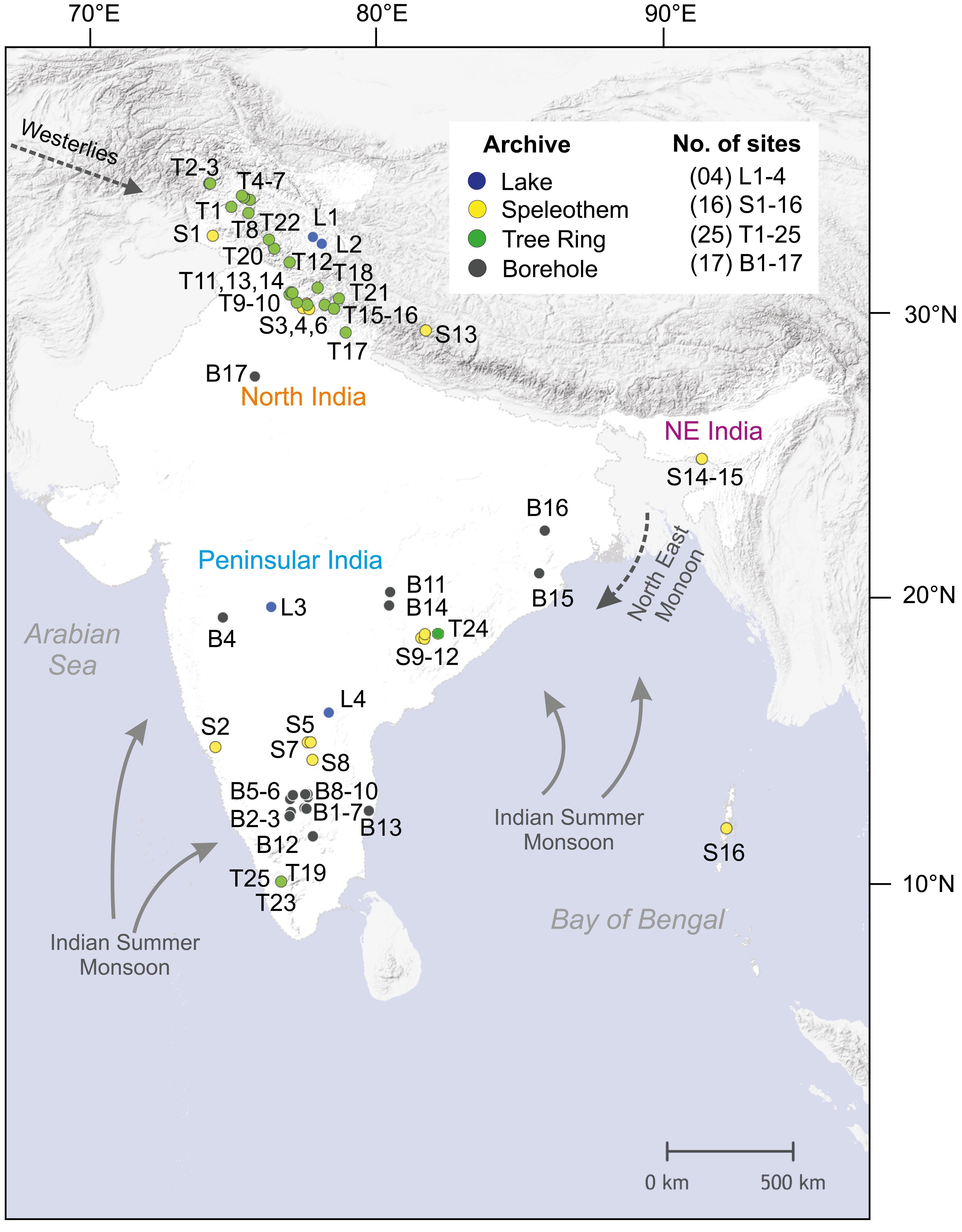
Figure 1: Spatial distribution of paleoclimate records from the terrestrial Indian region available in NOAA, PANGAEA, and Neotoma repositories and made available by PAGES working groups. Detailed information of archives, records and sources are given in the table hosted at https://doi.org/10.5281/zenodo.4292977. |
Distribution of accessible terrestrial Indian paleoclimate data
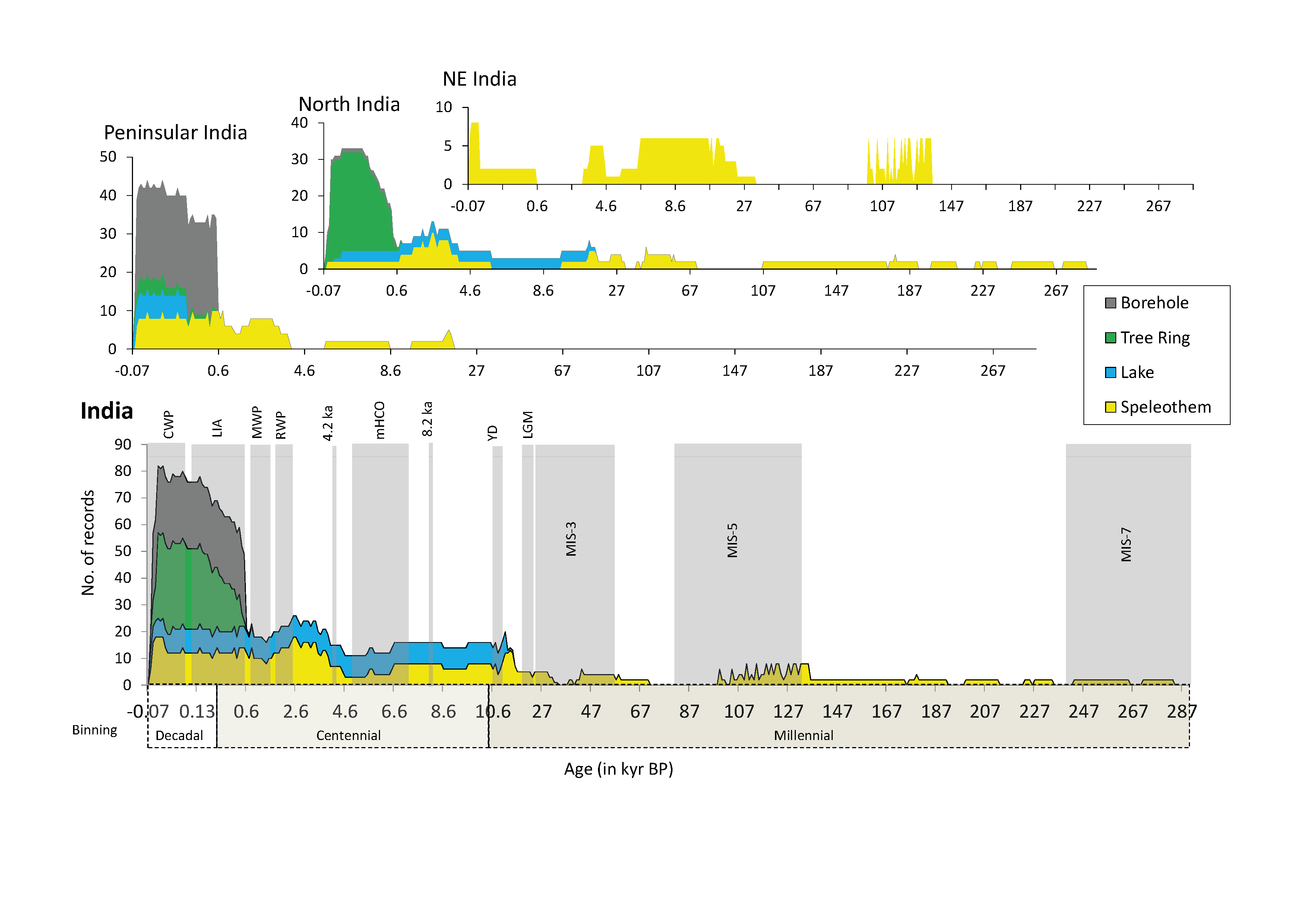
The terrestrial Indian region has been geographically divided into north, northeast, and peninsular subregions, which have distinct sources of moisture and climates (Fig. 1). Paleoclimate records in databases and repositories are available from speleothem, lake, tree-ring, and borehole archives. North and peninsular India have a high density of paleoclimate records from multiple archives. Northeast India has only speleothem records. Records from the central Indian Indo-Gangetic plain are conspicuously lacking. The geologically oldest proxy records are from speleothems, with the north Indian Bittoo cave record extending intermittently to ~280,000 years before present (Fig. 2). Most of the remaining speleothem records from all three regions cover the last ~30,000 years. Lake records cover the last ~15,000 years, while tree-ring and borehole records cover the last ~500 years.
The NOAA repository hosts the highest number of tree-ring standard-growth index and isotope records, all borehole records (which are part of a single study), and a few speleothem stable isotope and trace element records (Table 1). The highest number of speleothem oxygen and carbon isotopic proxy records with standardized data and metadata have been made available by the PAGES working group Speleothem Isotope Synthesis and AnaLysis (SISAL) as sql and csv files. Lake records can be found in the PANGAEA and Neotoma repositories. Many speleothem, tree-ring, borehole, and lake records covering the last 2000 years have been made available by the PAGES 2k Network with extended data and metadata in different formats in the NOAA repository and in FigShare.
| Data Source | Archive | No. sites | No. Entities | No. Proxy Records | Data access |
| Neotoma | Lake | 1 | 1 | 1 | Neotomadb https://www.neotomadb.org/ > Database Explorer > Scroll map to India > Advanced Search > Search by geopolitical unit> India |
| NOAA | Speleothem | 6 | 15 | 33 | NOAA https://www.ncdc.noaa.gov/paleo-search/ > Data type: speleothems > Advanced Search > Locations > Continent > Asia > Southcentral > India |
| Tree ring | 24 | 31 | 31 | NOAA https://www.ncdc.noaa.gov/paleo-search/ > Data type: Tree ring> Advanced Search > Locations> Continent > Asia > Southcentral > India | |
| Borehole | 17 | 17 | 17 | NOAA https://www.ncdc.noaa.gov/paleo-search/ > Data type: Borehole> Advanced Search > Locations> Continent > Asia > Southcentral > India | |
| PAGES | Speleothem | 16 | 38 | 75 | PAGES http://pastglobalchanges.org/ > Data: databases > SISAL |
| PANGAEA | Lake | 3 | 3 | 8 | PANGAEA https://www.pangaea.de/ > All Topics > India |
| Speleothem | 1 | 1 | 2 | PANGAEA https://www.pangaea.de/ > All Topics > India | |
|
Table 1: Data accessibility in NOAA, PANGAEA, and Neotoma repositories and made available by PAGES working groups. Each entity indicates the individual lake-core/speleothem/borehole/tree-ring master chronology, and the proxy record indicates a measurement that can be used individually to provide climatic/environmental information (for example, oxygen isotopes, tree ring standard growth index, palynology). |
|||||
 |
|
Figure 2: Temporal distribution of paleoclimate records from the terrestrial Indian region. CWP: Current Warm Period; LIA: Little Ice Age; MWP: Medieval Warm Period; RWP: Roman Warm Period; 4.2 ka: 4.2 ka Dry event; mHCO: Mid-Holocene Climate Optimum; 8.2 ka: 8.2 ka event; YD: Younger Dryas; LGM: Last Glacial Maxima; MIS 3, 5 and 7 are Marine Isotope Stages. |
Opportunities and gaps
Speleothem oxygen isotopic records provide sub-decadal- to millennial-scale information of past circulation and monsoon conditions from the terrestrial Indian region (Kaushal et al. 2018). They can be used for isotope-enabled climate model-data comparisons to improve our process-based understanding of controls on the monsoon (Battisti et al. 2014) and increase confidence in the ability of climate models to predict future changes (Schmidt 2010). As of yet, only very limited spectral analysis of existing oxygen and carbon isotopic records from the terrestrial Indian region has been performed to identify sub-decadal- and decadal-scale monsoon patterns (Midhun et al. 2020). Similarly, speleothem carbon isotopic and trace element records are increasingly being used to understand past changes in local climatic and environmental conditions in regions around the globe (Fairchild and Treble 2009; Fohlmeister et al. 2020); however, there are currently few measurements of trace elements or analysis of these proxy data from the Indian region.
Tree-ring growth indices produced from conifer and teak trees provide the highest resolution information of terrestrial climate in India. Tree-ring data are useful for continental-scale reconstruction and analysis of past droughts and temperatures (Cook et al. 2010; PAGES2k Consortium 2017). Millennium-long tree-ring chronologies developed in the terrestrial Indian region (Yadav et al. 2011; Yadav 2013) offer an opportunity to decipher centennial-scale climate variability and to understand prevailing climate during important phases such as the Medieval Warm Period, Little Ice Age, and Current Warm Period. The scarcity of trees with annually resolved tree rings is one of the main reasons for having only a few tree-ring datasets from peninsular India (Fig. 1). A "tree ring" defined based on the seasonality in the isotopic record of trees (Evans and Schrag 2004) could provide the necessary chronology to reconstruct past climate using trees lacking discernible growth rings. Such analysis can be used to decipher past variability in the frequency and intensity of the dry spells during monsoons (Managave et al. 2010), and in simultaneously reconstructing southwest and northeast monsoonal rainfall (Managave et al. 2011).
Lake sediments provide archives of regional to global climate change. Continuous sedimentation allows climatic variability to be assessed over several millennia through analysis of organic (e.g. pollen, carbon isotopes, total organic carbon, lipid biomarkers, diatoms) and inorganic (e.g. grain size, elemental chemistry, environmental magnetism; e.g. Rawat et al. 2015a, b; Sarkar et al. 2015) proxies. India hosts many natural lakes extending from the high-altitude alpine Himalayan regions to the tropical peninsula. Because most Indian lakes are non-varved and receive low sedimentation, they can provide semi-quantitative rainfall estimates only at centennial resolution. More than 76 lake records from India have been analyzed in the literature (Misra et al. 2019); however, as of yet only nine proxy records from four lakes have been made available in databases and repositories. A paleolimnological community-based effort is required to both produce new data from India's many lakes and increase the availability of previously collected lake-sediment records.
Summary
Our analysis suggests that paleoclimate work in the Indian region can be improved by (1) increasing the number and accessibility of lake-sediment records region-wide, (2) generating data from records that extend beyond the last 15,000 years, and (3) generating data from geographically under-represented subregions, such as the central Indian Indo-Gangetic plain. Combining information across the diverse proxy records in the repositories and databases will provide opportunities to assess factors influencing major moisture drivers and mechanisms associated with westerlies and the Asian monsoon system.
acknowledgements
PS acknowledges funding from FAPESP Postdoctoral grant 2019/11364-0.
affiliations
1Asian School of the Environment, Nanyang Technological University, Singapore
2Department of Civil Engineering, Gharda Institute of Technology, Ratnagiri, India
3Instituto Oceanográfico, Universidade de São Paulo, Brazil
4Wadia Institute of Himalayan Geology, Dehradun, India
5Indian Institutes of Science Education and Research, Pune, India
contact
Nikita Kaushal: nikitagelogistgmail.com
references
Battisti DS et al. (2014) J Geophys Res Atmos 119: 11-997
Comas-Bru L et al. (2019) Clim Past 15: 1557-1579
Cook ER et al. (2010) Science 328: 486-489
Dasu T, Johnson T (2003) Exploratory Data Mining and Data Cleaning John Wiley & Sons, 203 pp
Evans MN, Schrag DP (2004) Geochim Cosmochim Acta 68: 3295-3305
Fairchild IJ, Treble PC (2009) Quat Sci Rev 28: 449-468
Fohlmeister J et al. (2020) Geo Cosmo Acta 279: 67-87
Kaushal N et al. (2018) Quaternary 3: 29
Managave SR et al. (2010) Geophys Res Lett 37: L05702
Managave SR et al. (2011) Clim Dyn 37: 555-567
Midhun M et al. (2020) Geophys Res Lett: 47, e2020GL089515
Misra P et al. (2019) Earth-Sci Rev 190: 370-397
Owen R et al. (2018) Comput Geosci 119: 115-122
PAGES2k Consortium (2017) Sci Data 4: 170088
Rawat S et al. (2015a) Quat Sci Rev 114: 167-181
Rawat S et al. (2015b) Palaeogeogr Palaeoclimatol Palaeoecol 440: 116-127
Sarkar S et al. (2015) Quat Sci Rev 123: 144-157
Schmidt GA (2010) J Quat Sci 25: 79-87
Tardif R et al. (2019) Clim Past 15: 1251–1273
Yadav RR (2013) J Geophys Res Atmos 118: 4318-4325
Yadav RR et al. (2011) Clim Dyn 36: 1545-1554
links
PAGES2k Consortium (2017):
NOAA: https://www.ncdc.noaa.gov/paleo/study/21171
FigShare: https://figshare.com/collections/A_global_multiproxy_database_for_temperature_reconstructions_of_the_Common_Era/3285353
SISAL database v2.0: researchdata.reading.ac.uk/256/
NOAA repository: https://www.ncdc.noaa.gov/data-access/paleoclimatology-data/datasets
PANGAEA repository: https://pangaea.de/
Neotoma database: https://www.neotomadb.org/
SISAL working group: pastglobalchanges.org/sisal
PAGES 2k Network: pastglobalchanges.org/2k
Allison E. Lawman1,2, J.W. Partin2 and S.G. Dee1
Proxy system models provide a tool to link paleoclimate proxy data with instrumental observations or climate model output. Recent advances in coral proxy system modeling cement the fidelity of tropical Pacific corals in recording changes in El Niño-Southern Oscillation variability.
Reconstructing ENSO variability using corals
The El Niño-Southern Oscillation (ENSO) is a tropical climate phenomenon that has global impacts on temperature and rainfall patterns. Given its role as the leading mode of interannual variability and the socioeconomic impacts associated with these events, it is of paramount importance to understand how ENSO may change in the future with anthropogenic warming. Tropical climate variability is a source of notable uncertainty in future climate projections (Bellenger et al. 2014; Collins et al. 2010). While simulations provide insight into how ENSO may behave in a warmer world, they often lack critical constraints from physics (Collins et al. 2013), and require independent validation to assess the accuracy of a model's performance. This motivates the study of past ENSO variability during periods when Earth experienced different conditions compared to today's rapidly warming climate.
Corals are a paleoclimate archive well-suited for studying ENSO variability, as they store decades to centuries of sub-annually resolved proxy climate information from the tropics (Fairbanks et al. 1997; Lough 2010). Modern corals serve to calibrate proxies with the instrumental record, while fossil corals provide snapshots of interannual variability during pre-industrial times. In particular, the ratio of strontium to calcium (Sr/Ca) and the oxygen isotopic composition (δ18O) of the coral skeleton are well-established proxies for oceanic conditions. Coral Sr/Ca varies in response to changes in sea-surface temperature (SST), while coral δ18O jointly records changes in SST and the ratio of the oxygen isotopic composition of seawater to salinity (δ18Oseawater/salinity; Corrège 2006; Lough 2010).
Proxy system modeling as a tool to quantify uncertainties
On interannual timescales, corals from the tropical Pacific are influenced by ENSO, local variability, and how the coral itself records climate information. Since corals are widely used to reconstruct paleo-ENSO variability, it is critical to quantify how these factors impact estimates of interannual variability in proxy records. A proxy system model (PSM) is a tool that quantifies sources of uncertainty by mathematically modeling how different processes impact a climate signal that emerges from the proxy data (Dee et al. 2015; Evans et al. 2013). Paleoclimate proxy data is often used to reconstruct climate variables, such as temperature, via empirically determined calibration equations. Alternatively, a PSM can use observed or simulated climate information and generate a forward-modeled time series of what a hypothetical proxy under those conditions would record, i.e. a "pseudoproxy". This calculation translates the climate signal to a proxy signal and considers ways by which the proxy alters the input signal. PSMs thus provide a means to directly compare proxy data and instrumental observations or climate model output in the same units.
 |
|
Figure 1: Percent difference in standard deviation (SD) between pseudocoral (A) SSTSr/Ca and (B) δ18O anomalies perturbed with variable growth rates, analytical/calibration errors, and the age modeling algorithm (n = 100 realizations), and the original, unperturbed environmental input. The white box outlines the Niño 3.4 region. The model output used here and in Figure 2 is from the CESM-LME 850 control simulation (Otto-Bliesner et al. 2016). Figure reproduced with permission from Lawman et al. (2020). |
Coral proxy system modeling work by Thompson et al. (2011) provides an example of a transfer function used to forward model "pseudocoral" δ18O as a linear combination of SST and δ18Oseawater/salinity. This sensor model has since been used for many purposes, including comparing coral δ18O records with pseudocoral time series generated from instrumental observations and historical climate model simulations (Thompson et al. 2011), and quantifying errors in coral-inferred estimates of ENSO amplitude (Russon et al. 2015) and variability (Stevenson et al. 2013). Our recent coral PSM builds on this and earlier studies by adding new features, called sub-models, into an existing coral PSM framework (Lawman et al. 2020). We use temperature and salinity output from the Community Earth System Model Last Millennium Ensemble (CESM-LME; Otto-Bliesner et al. 2016) to model pseudocoral δ18O and SST derived from coral Sr/Ca (SSTSr/Ca) and quantify how uncertainties associated with assumptions about (1) analytical and proxy-calibration errors, (2) variable coral growth rates, and (3) coral age-depth modeling impact estimates of interannual variability, here defined at the standard deviation of δ18O and SSTSr/Ca anomalies.
Our results demonstrate that calibration and analytical errors increase estimates of interannual variability in coral geochemical records, whereas variations in growth rates, when combined with certain age modeling assumptions, systematically decrease estimates of interannual variability. When all three sub-models are coupled, we find that such factors can measurably change the standard deviation of δ18O and SSTSr/Ca anomalies on the order of 10-30% compared to the original, and that the relative importance of each sub-model is specific to individual sites (Fig. 1). We attribute the degree of site-specific changes in interannual variability to the tradeoff between the strength of the interannual signal (ENSO) and the amplitude of the SST annual cycle at a given site.
 |
|
Figure 2: Correlation between Niño 3.4 SST anomalies and values at each grid point. Monthly Niño 3.4 SST anomalies correlated with monthly (A) SST anomalies and (B) δ18O generated using the sensor model of Thompson et al. (2011). The 20-year running SD of Niño 3.4 SST anomalies (i.e. decadal+ changes in ENSO variability) correlated with (C) SST and (D) pseudocoral δ18O anomalies. The 20-year running SD of Niño 3.4 SST anomalies correlated with (E) SSTSr/Ca and (F) pseudocoral δ18O anomalies perturbed by the three coral PSM sub-models. Statistically significant correlations (p < 0.01) are stippled. The gold diamond (C-F) indicates the average correlation coefficient for the Niño 3.4 region (white box). Figure reproduced with permission from Lawman et al. (2020). |
The PSM is a useful tool for not only quantifying how various coral uncertainties manifest locally at individual sites, but also how they impact a coral's ability to broadly capture changes in ENSO variability. The Niño 3.4 region has been identified as a "center of action" for ENSO (Fig. 2a-b), and the month-to-month correlation between SST and SST anomalies over this region is a common metric for assessing the ENSO sensitivity at a site. However, fossil corals with absolute age errors on the order of 1% preclude such a precise month-to-month reconstruction back in time. To address this limitation, we investigate how local δ18O and SSTSr/Ca variability track changes in ENSO variability on decadal and greater timescales (decadal+) using the correlation between the running standard deviation of pseudocoral δ18O and SSTSr/Ca anomalies with Niño 3.4 SST anomalies (Fig. 2c-d). Although the correlations are, as expected, smaller (Fig. 2e-f) than the original inputs not processed with the three PSM sub-models, the temporal relationship between changes in the pseudocorals and changes in Niño 3.4 SST variability is broadly preserved. Many circum-Pacific locations, particularly those near coral atolls, demonstrate statistically significant correlations with ENSO changes. This highlights the ability of corals from across the tropical Pacific to capture decadal+ changes in ENSO variability.
Future perspectives
Although different processes and assumptions inherent to paleoclimate studies may impact estimates of interannual variability recorded by corals, our recent PSM work highlights the strength of corals in their ability to capture decadal+ changes in ENSO variability. It is most appropriate to compare coral geochemical data with instrumental or climate model output processed through a PSM, as it places the two types of data on a more level playing field. To help facilitate such comparisons, our new PSM sub-models are publicly available to the climate community via a GitHub repository (https://github.com/lawmana/coralPSM). Future work comparing coral geochemical data with climate model observations translated to coral units using a process-based PSM will be a key step toward reconciling differences between models and coral geochemical observations. It is our hope that sharpening our data-model comparisons for the tropical oceans will allow us to refine the implementation of important physical processes in models, thereby reducing uncertainties in future ENSO projections.
affiliations
1Department of Earth, Environmental and Planetary Sciences, Rice University, Houston, TX, USA
2Institute for Geophysics, The University of Texas at Austin, USA
contact
Allison E. Lawman: Allison.Lawmanrice.edu
references
Bellenger H et al. (2014) Clim Dyn 42: 1999-2018
Collins M et al. (2010) Nat Geosci 3: 391-397
Corrège T (2006) Palaeogeogr Palaeoclimatol Palaeoecol 232: 408-428
Dee S et al. (2015) J Adv Model Earth Syst 7: 1220-1247
Evans MN et al. (2013) Quat Sci Rev 76: 16-28
Fairbanks RG et al. (1997) Coral Reefs 16: S93-S100
Lawman AE et al. (2020) Paleoceanogr Paleoclimatol 35: e2019PA003836
Lough JM (2010) WIREs Clim Change 1: 318-331
Otto-Bliesner BL et al. (2016) Bull Am Meteorol Soc 97: 735-754
Russon T et al. (2015) Geophys Res Lett 42: 1197-1204
Magdalena Fuentealba![]() 1,2, C. Latorre1,2, M. Frugone-Álvarez1,2, P. Sarricolea3 and B. Valero-Garcés4
1,2, C. Latorre1,2, M. Frugone-Álvarez1,2, P. Sarricolea3 and B. Valero-Garcés4
Stable nitrogen isotopes on organic matter from lake sediments in central Chile combined with reconstructions of land-use and cover change show the magnitude of human influence and the onset of the Great Acceleration.
The Anthropocene in central Chile
The Anthropocene has been proposed as a new geological epoch where humankind has become a major driver of the Earth's biosphere and surface processes to an extent that can be readily observed in the sedimentary record (Crutzen and Stoermer 2000). The Anthropocene Working Group of the International Commission on Stratigraphy (https://stratigraphy.org) has recently defined the starting point of the Anthropocene at around 1950 CE, which marks a period of dramatic change in magnitude and rate of the global human activity (the Great Acceleration; Zalasiewicz et al. 2019). However, this date remains a point of contention as agricultural impacts (and associated impacts) have been increasing throughout the Holocene (Ellis et al. 2016; Ruddiman 2019; Zalasiewicz et al. 2019).
Nitrogen, carbon, and phosphorus biogeochemical cycles can all affect primary productivity, and their alteration can cause serious environmental problems such as cultural eutrophication and contamination of terrestrial and aquatic ecosystems. Records of past variations in biogeochemical cycles can help unravel the timing and intensity of the Anthropocene (Wolfe et al. 2013; Zalasiewicz et al. 2019). Humans have had important impacts on the landscape of the Pacific coast of central Chile at least since the Spanish colonial period (16th to 18th centuries). These have been associated with agriculture development, increased fire regimes, and deforestation of native species (Armesto et al. 2010; Gayo et al. 2019). Nowadays, most human impact is related to increasing demands for tree plantations of exotic species (especially Pinus radiata and Eucalyptus globulus).
 |
|
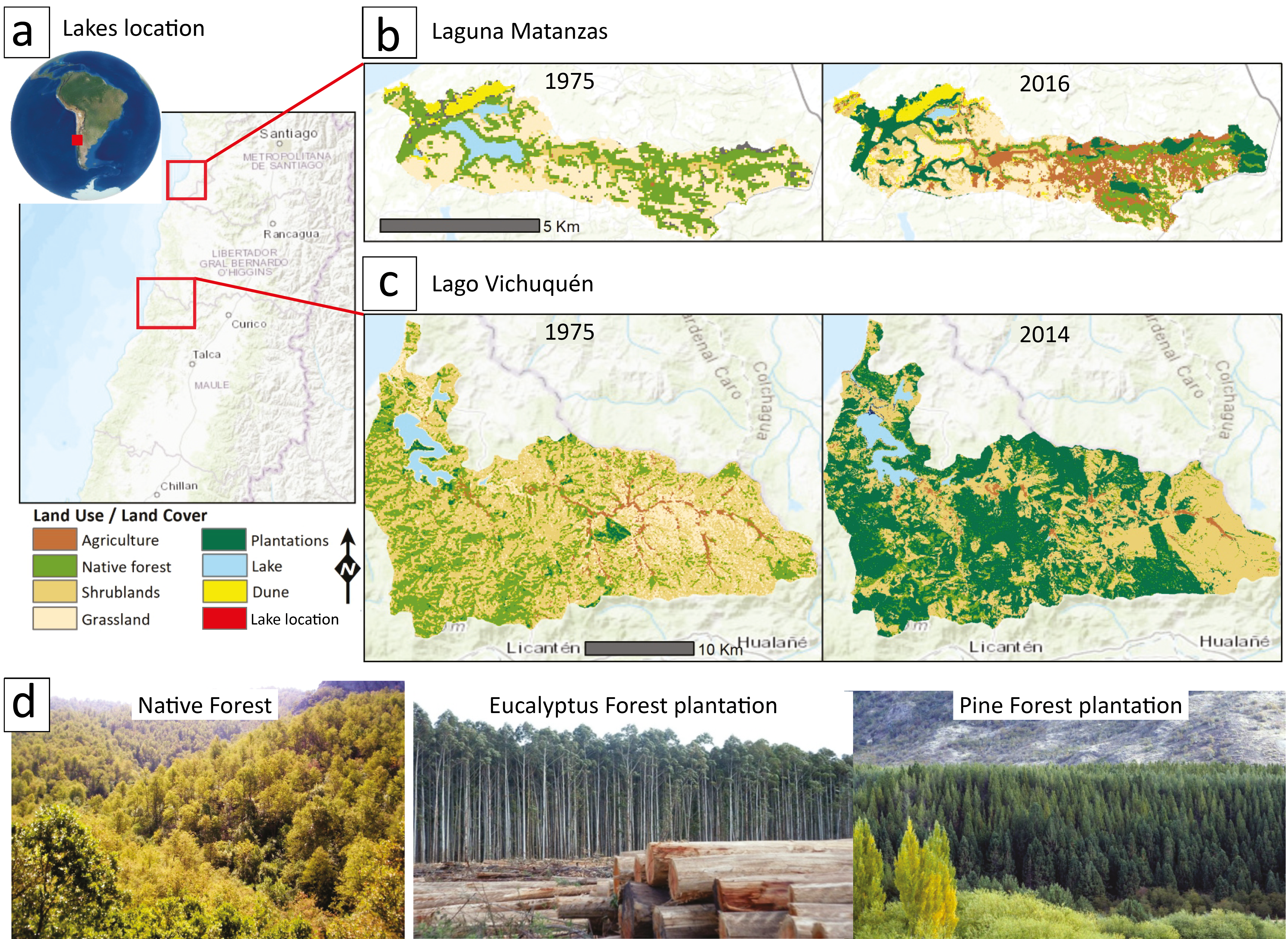
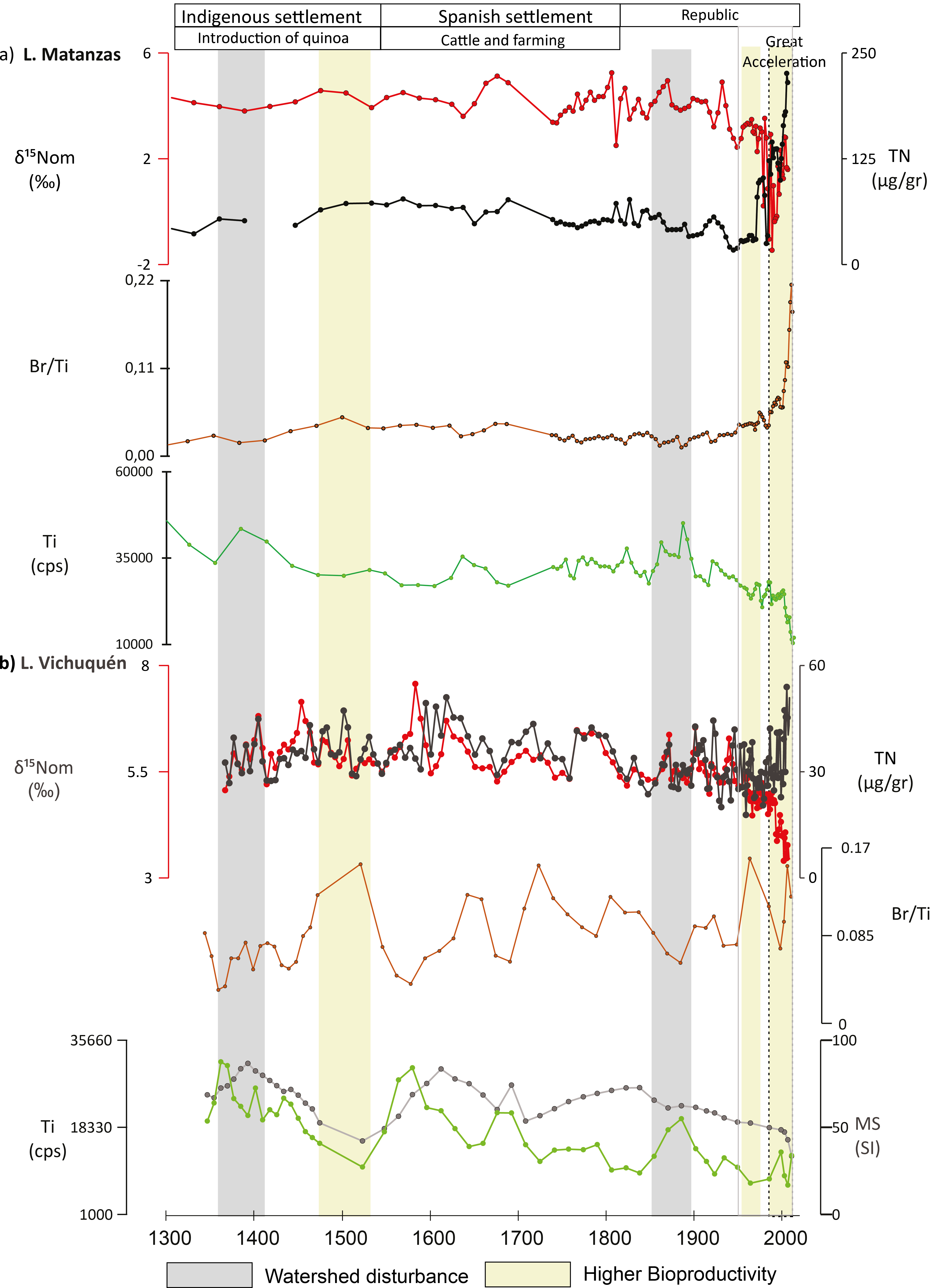
Figure 1: (A) Location of Laguna Matanzas and Lago Vichuquén in South America. (B) and (C) Land-use and cover changes in both watersheds from 1975 CE and 2014 (Lake Vichuquén) and 2016 (Lake Matanzas) CE (map sources: Esri, HERE, Garmin, World Topographic Map). (D) Examples of native forests compared with tree plantations in central Chile. |
We studied two coastal lakes from central Chile to examine the structure and timing of the Anthropocene and the onset of the Great Acceleration. For this, we compared land-use and cover change (LUCC) with stable nitrogen isotopes on lake organic matter (δ15Nom) and multiproxy analyses from lake sediments. The Laguna Matanzas watershed (30 km2 surface area; Fig. 1b) was mainly occupied by native forest and grassland areas in 1975 CE, but by 2016 CE, tree plantations covered a third of the total area. At Lago Vichuquén, only 1% of the watershed (535.3 km2 surface area; Fig. 1c) was covered by exotic tree plantations in 1975 CE; however, these increased up to 66% by 2016 CE.
Watershed-lake dynamics inferred from the sediment record
The Br/Ti ratios in lake sediment from coastal lakes of central Chile are commonly elevated with high organic carbon content, indicating higher lake productivity (Frugone-Álvarez et al. 2017; Fuentealba et al. 2020). Similarly, fluctuations in δ15Nom in lake records have been used as an indicator of changes in paleoproductivity and/or watershed disturbances (Das et al. 2009; Torres et al. 2012).
Historic LUCC in the Laguna Matanzas watershed began during the Spanish colonial period with a Jesuit settlement in 1627 CE and the development of a livestock ranch. After the Jesuits were expelled from South America in 1778 CE, the ranch reached more than 40,000 head of cattle around 1800 CE. During this first period, the watershed-lake dynamics displayed moderate-to-low productivity (Br/Ti; Fig. 2) with elevated sediment input as indicated by our geochemical proxies (Ti; Fig. 2; Fuentealba et al. 2020). Sediment δ15Nom values from the 14th to 19th centuries were relatively high, probably reflecting N inputs from cow manure and soil particles that typically generate higher sediment δ15Nom values (Fig. 2). From the 19th to mid-20th centuries, these overall patterns did not change. The δ15Nom and total nitrogen (TN) values were slightly lower than during the Colonial Period and changes in both were in phase and relatively synchronous.
 |
|
Figure 2: Anthropogenic influences on changes in the N availability and lake productivity during the last six centuries in central Chile (Laguna Matanzas and Lago Vichuquén). Higher sediment δ15Nom values (red line) covaried with the TN (black line), indicating higher lake productivity (Br/Ti) after periods of watershed disturbance (magnetic susceptibility, Ti). |
The implementation of the Chilean Forestry Law Decree of 1931 (DFL n°265) contributed to a strong development of forestry that was coeval with decreased sediment input (low Ti) from the watershed and slightly increased lake productivity (higher Br/Ti). Until the 1970s, the Laguna Matanzas watershed was mostly covered by native forest, and grassland areas were intended for livestock grazing (Fig. 1; Fuentealba et al. 2020). From the 1980s onwards, sediment δ15Nom values decreased, reaching their lowest values in the entire sequence at ca. 2000 CE. During the 21st century, the sediment δ15Nom values increased in tandem with the highest TN values seen in the record (Fig. 2). The increased lake productivity, the sharp change in δ15Nom trend, and the decreased sediment input during the last few decades has been synchronous with the replacement of intensive livestock grazing by intensive agriculture and forestry practices (Fuentealba et al. 2020).
Land use during the colonial period in Lago Vichuquén was characterized by agriculture, cattle ranching, and mining under the Encomienda (feudal) system (Vidal and Ramírez 1985). Historical documents show that before 1580 CE, the Vichuquén watershed was occupied by Indigenous communities dedicated to small-scale farming, extracting wood, and mining activities. The sediment δ15Nom values from this period covary with TN, indicating pulses of enhanced N input from the watershed were likely linked to an increase in land use and sediment input (indicated by changes in magnetic susceptibility and Ti content in Fig. 2).
From the onset of the 19th to the mid-20th centuries, δ15Nom and TN values decreased slightly, most likely related to lowered sediment input from the watershed until the second half of the 19th century. In contrast, the last part of the 20th century witnessed accelerated changes in the watershed as native forests, meadows, and shrublands were quickly replaced by exotic tree plantations (Fig. 1). These changes were synchronous with a major regime shift in the nitrogen cycle as observed by an increase in TN along with lowest δ15Nom values seen in the record.
The δ15Nom lake-sediment record as a tracer of the Anthropocene
Numerous records indicate that the onset of the Great Acceleration in the Northern Hemisphere was around 1950 CE (e.g. Holtgrieve et al. 2011; Rose 2015; Zalasiewicz et al. 2019). However, the timing and magnitude of human activities were likely different between and within the hemispheres. Our results from Laguna Matanzas and Lago Vichuquén show elevated TN concentrations in tandem with the lowest sediment δ15Nom values in the entire record during the 1980s (Fig. 2). Thus, human activities associated with exotic tree plantations clearly had major impacts on the watershed-lake dynamics and nitrogen cycling in central Chile, several decades after the onset of the Great Acceleration. Although nitrogen dynamics respond to limnological processes as well, both lakes crossed a critical threshold, not seen in more than three centuries, during the 1980s due to regional processes associated with national policy changes and government subsidies.
Our study shows that during the historical period in Chile it is not necessarily the presence of human activities per se that alters watershed-lake dynamics, but rather the magnitude and intensity of such activities associated with major land-use and cover changes. The increase in tree plantations and intensive agriculture over the last 40 years (since the late 70s and early 80s) has contributed to a shift in sediment input and nutrient transfer to Laguna Matanzas and Lago Vichuquén, affecting productivity in a way that is unprecedented during the last 500 years. Though the Anthropocene and the Great Acceleration have been formally defined globally, we note that local and regional impacts often produce major changes in sedimentary records that are often at odds with these definitions. In the case of heavily populated central Chile, these impacts began with intense activity associated with extensive exotic tree plantations that started in the 1980s, three decades after the beginning of the Great Acceleration.
affiliations
1Pontificia Universidad Católica de Chile, Santiago, Chile
2Institute of Ecology and Biodiversity (IEB), Santiago, Chile
3Universidad de Chile, Santiago, Chile
4Instituto Pirenaico de Ecología (IPE-CSIC), Zaragoza, Spain
contact
Magdalena Fuentealba: magdalena.fuentealbagmail.com
references
Armesto J et al. (2010) Land Use Policy 27: 148-160
Crutzen P, Stoermer EF (2000) Glob Change Newsl 41: 17-18
Das B et al. (2009) J Paleolimnol 42: 167-181
Ellis E et al. (2016) Nature 540: 192-193
Frugone-Álvarez M et al. (2017) J Quat Sci 32: 830–844
Fuentealba M et al. (2020) Sci Rep 10: 5864
Gayo E et al. (2019) Elementa 7: 15
Holtgrieve G et al. (2011) Science 334: 1545-1548
Rose N (2015) Env Sci Technol 49: 4155-4162
Ruddiman W (2019) Prog Phys Geogr 43: 345-351
Torres IC et al. (2012) J Paleolimnol 47: 693-706
Vidal S, Ramírez O (1985) Vichuquén: 400 años. La Prensa press, 255 pp
Christine A. Omuombo![]()
Paleo records from Lake Nkunga show that climatic and environmental changes in this region were gradual and subtle during the last millennium. We highlight the importance of sedimentary records in providing a baseline for future conservation efforts on Mt. Kenya.
The last few hundred years have been characterized by increasing anthropogenic utilization of land and land-based resources, resulting in significant changes to the landscape and ecosystems, both in their structure and function. Baseline climate and land-use parameters can be deduced from climate-sensitive lakes with a high degree of reliability (Olago and Odada 2004). Forest cover, in particular, has seen unprecedented disturbances in recent times due to human occupation and modifications in land-use patterns. The overprint of anthropogenic influence on the climate signal is difficult to decipher without clear records of long-term change. Lake sediments within forests are ideal proxy archives to investigate the linkages between natural and anthropogenic factors. In the last millennium, evidence of climate and environmental change from decadal to centennial scales (Tierney et al. 2013; Verschuren et al. 2000) reveal floral and aquatic transformations that can be used as baselines for our decision-making regarding the conservation of our natural resources.
Climate context and human impact during the last millennium over East Africa
During the Late Holocene, East Africa experienced warm and moist conditions (Kiage and Liu 2006), punctuated by two key climatic events: The Medieval Climate Anomaly (MCA; 950–700 cal yr BP) and the Little Ice Age (LIA; 700–100 cal yr BP), observable in proxy records from many sites. The MCA was dry with low lake levels and was synchronous among various sites within a relatively narrow time window. In contrast, the timing of the LIA is highly variable, with the first phase of the LIA corresponding to maximum lake levels due to increased precipitation and the second phase displaying lake-level regressions punctuated by centennial- and decadal-scale droughts (Verschuren et al. 2000). These climatic events coincided with the expansion and settlement of various communities and are therefore difficult to isolate from anthropogenic impacts on the ecosystem responses.
The expansion of trade routes between the interior and the coast of East Africa in the 19th century played a key role in land-cover modification. The spread of domesticated crops from different parts of the world such as East Asia (banana, rice, and cassava) and South and Central America (maize, tomato, and avocado) have been archived in sedimentary records documenting population expansion in the region (Marchant et al. 2018). However, comprehensive datasets describing both the anthropogenic and climate influences on land use only exist for a handful of sites in East Africa, such as lakes Victoria and Naivasha in Kenya.
The Mt. Kenya highlands during the last millennium
 |
|
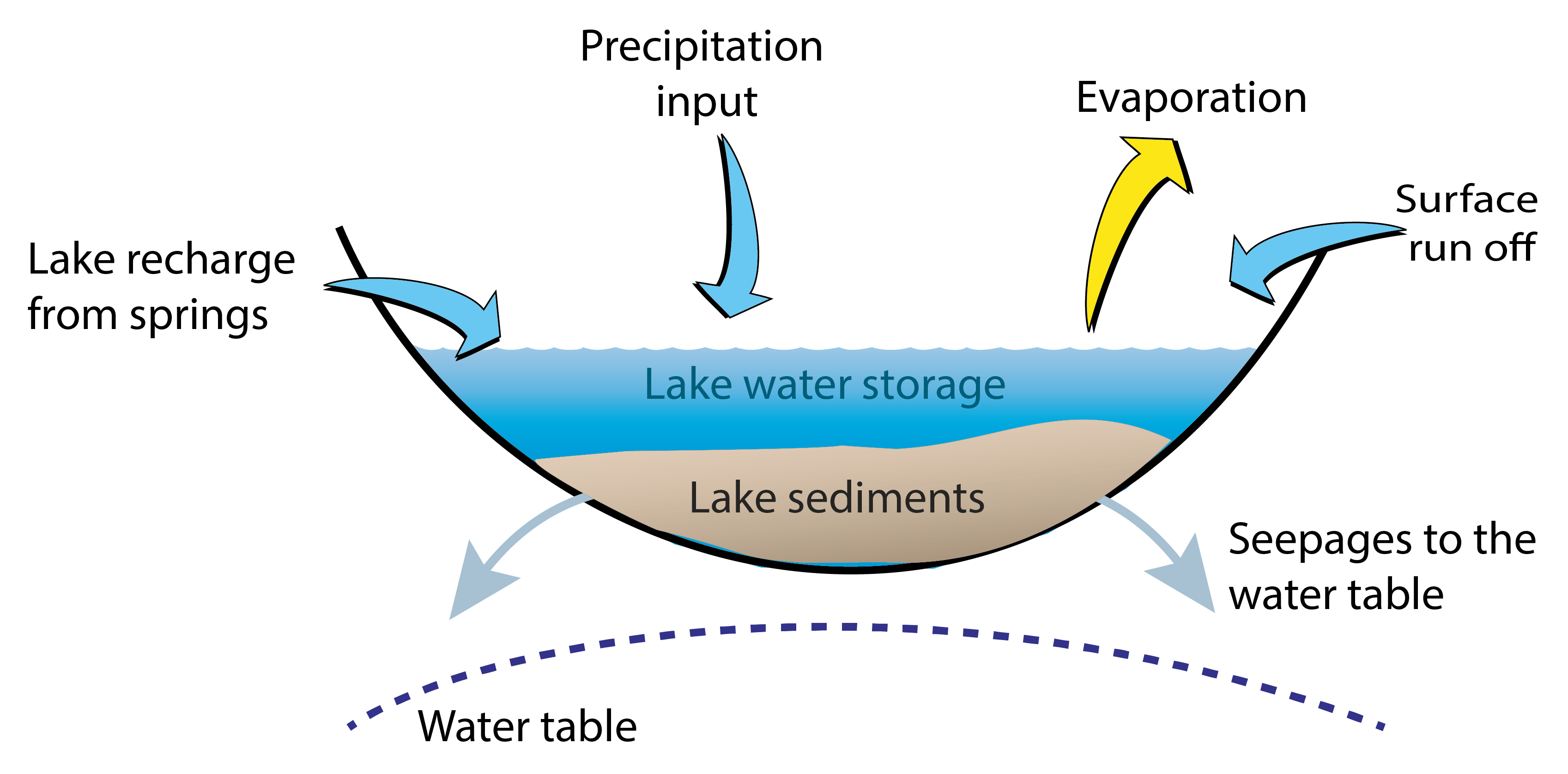
Figure 1: A simplified lake water budget model for Lake Nkunga. |
Mt. Kenya Forest is a protected area in the East Africa highlands. Several crater and glacial lakes located in different ecological zones of the mountain have been studied to better understand the climatic and environmental signals within their sediments. One of the lakes within Mt. Kenya Forest, Sacred Lake (2350 m asl), hosts the longest records of climate and environmental change spanning the period from 115,000 cal yr BP to present (Olago 2001). During the 20th century the forested catchment areas were converted to agriculturally productive lands for commercial and subsistence farming. As a consequence, an explosion of the human population relying on the utilization of forest-based resources and overuse of arable and pasture lands is an increasing threat to the present-day forest ecosystem.
The first written records of human occupation of the Mt. Kenya region by local communities was about 200 cal yr BP. The extent of their invasion into the montane forest region is not well known (Ndichu 2009); what has been established is that this expansion coincided with periods of conflict over natural resources and civil wars during decadal-scale droughts (Verschuren et al. 2000). Therefore, it is possible that the anthropogenic signal for the last two centuries from this region, detected through the presence of agricultural traces in the sedimentary record, may be overestimated, requiring further analysis to better understand the observed changes.
Lake Nkunga is one of the shallow crater lakes on the northeastern slopes of the mountain located at the equator at 1780 m asl and is located 10 km below Sacred Lake (Omuombo et al. 2020). Previous studies from this lake indicate that sedimentation resumed during the Late Holocene after a hiatus from 30,000–1350 cal yr BP (Olago et al. 2000). The lake has since persisted as a permanent water body archiving sediment over the last millennium. The lake exhibits swamp-like conditions due to its shallow depth (1.9 m on average) and is recharged by precipitation and springs emanating from fissures located at higher altitudes to the east and west and has no known outlet (Fig. 1). We examined a short 89-cm core from this lake and carried out various biogeochemical analyses (mineralogy, magnetic susceptibility, and organic and elemental geochemistry) to decipher the lake responses to climatic and environmental changes during the last millennium (Omuombo et al. 2020).
 |
|
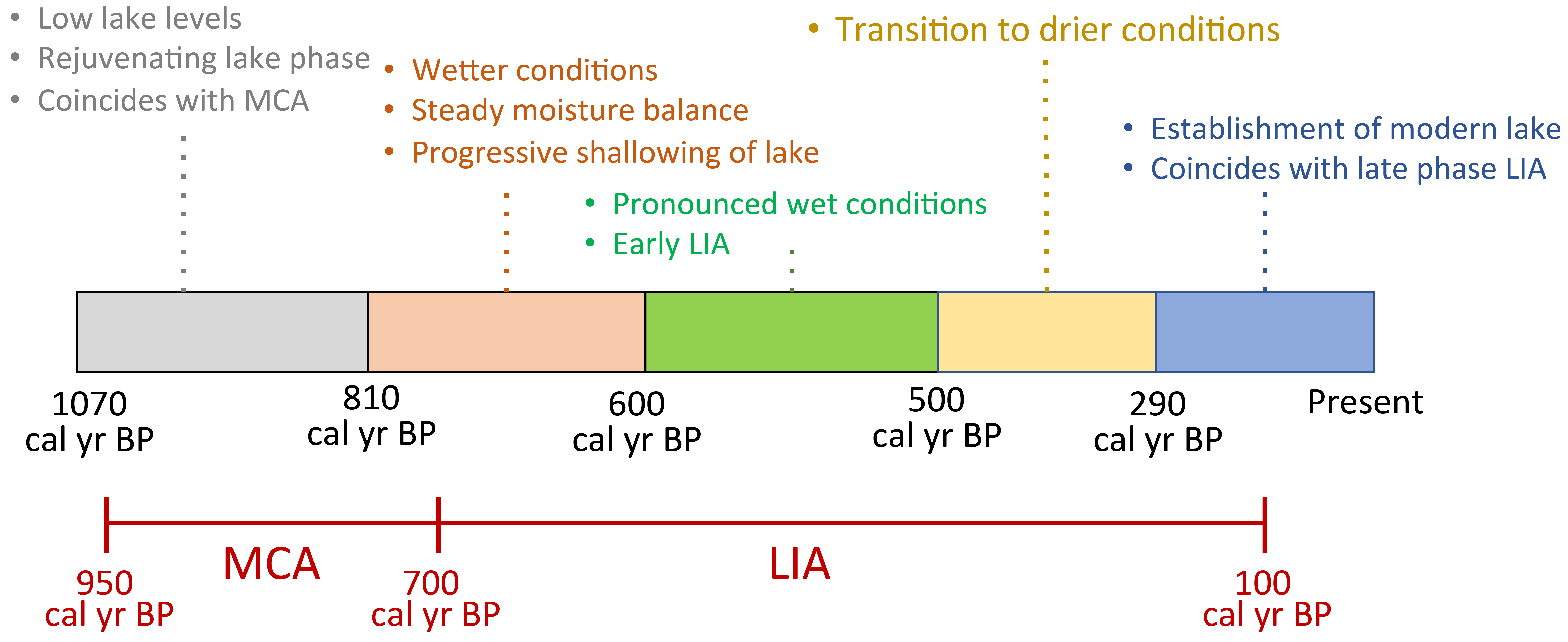
Figure 2: The interpretation of sedimentary archives from Lake Nkunga (sketch not to scale). |
The hydrological record commences with a warm MCA that coincides with a lake rejuvenation phase and exhibits characteristics signifying a low lake level (Fig. 2). Post MCA, a transition to wetter conditions within the first phase of the LIA is apparent between 600–500 cal yr BP (Fig. 2). Peak sediment influx and the development of swamp conditions (Omuombo et al. 2020) are observed during this time. A relatively stable lake level from 500–290 cal yr BP that has persisted to the present day shows subtle responses to drier conditions. Charcoal particles were visible in the sediments during this stable period, but the link to either anthropogenic or natural fires is yet to be resolved. Anthropogenic influence in our sedimentary record cannot be excluded, even though the first documented human occupation of Mt. Kenya was shortly after this period (ca. 200 cal yr BP). The lake has not changed significantly since 290 cal yr BP, perhaps pointing to the vital role of groundwater recharge from springs located above the lake in stabilizing lake levels.
The role of paleo information in conservation for Mt. Kenya
Lake Nkunga lies at the border of the dry montane forest zone of Mt. Kenya and a human occupation area. It serves as a water source for the villages around it and the wildlife within the Mt. Kenya Forest ecosystem. Recently, concerns were voiced regarding the terrestrialization of the lake due to the presence of reeds and floating mats of water lilies, sedges, and ferns that have restricted access to lake water. While catchment erosion and weathering processes from anthropogenic activities play a significant role in sediment supply in lakes, our record shows that from 290 cal yr BP to present, the sedimentation rate has declined from 0.4 cm/yr to a constant rate of 0.3 cm/yr. The current efforts to reclaim the lake include weed control and the establishment of an ecotourism site through the development of picnic areas, camping sites, and nature trails to increase community income.
Continued use and future development of Lake Nkunga's forested catchment need to be considered in the context of long-term lake-level changes and internal processes. The lack of a distinct anthropogenic signal from the Lake Nkunga record presents a baseline for the impact of future activities within the lake's catchment. Mt. Kenya Forest provides an important habitat for wildlife in the region, and thus conservation efforts are warranted. Our insights from the paleorecord of lake hydrology suggest that it is indeed important to conserve the forested catchment as a means to sustain the groundwater recharge to the springs that feed the lake. These springs play a critical role in managing the lake water budget (Fig. 1). The integration of paleo information into modern day management of natural resources is lacking despite the availability of such data from several additional sites in East Africa. Better informed governance and management of natural resources, especially during these unprecedented times of changing climatic and environmental conditions, is therefore possible. Consideration of past, present, and future changes could allow for the integration of catchment management policies critical for reaching sustainable development goals.
Acknowledgements
The author thanks D. Olago and D. Williamson for their helpful guidance and discussions. Support was provided by the TECLEA project, UMR METIS, UMR LOCEAN, and UMR CEREGE. Funding for this work was provided by IRD-DPF.
affiliation
Department of Geology, University of Nairobi, Kenya
contact
Christine Omuombo: omuombouonbi.ac.ke
references
Kiage LM, Liu KB (2006) Prog Phys Geogr 30(5): 633-658
Marchant R et al. (2018) Earth-Sci Rev 178: 322-378
Ndichu RW (2009) Drought and Flood Events and the Social-Economic and Political Impacts Experienced, 300-1900 AD. Sanctified Press, 384 pp
Olago DO (2001) Clim Res 17: 105-121
Olago DO et al. (2000) J Afr Earth Sci 30: 957-969
Omuombo C et al. (2020) Sci Afr: e00416
William Rapuc![]() , P. Sabatier
, P. Sabatier![]() and F. Arnaud
and F. Arnaud![]()
Human activities impact erosion and transport processes in catchments, hence disturbing paleoclimate recording. A thorough study of erosion patterns is therefore necessary to disentangle climate and human forcing when interpreting lake sediment-based flood chronicles.
Flood frequencies as a proxy of past extreme precipitation events
In the current context of global climate change, predicting the evolution of precipitation is particularly challenging: an increase of extreme events is expected globally due to the capacity of a warmer atmosphere to hold more water, although regional trends may differ (IPCC 2012). Assessing this requires the acquisition of long-term hydrological datasets (Wilhelm et al. 2019). As flood occurrence and magnitude are linked to precipitation-regime fluctuation through time, the establishment of regional flood chronicles from natural archives could be a key to evaluate the evolution of precipitation regimes on emerged land (Wilhelm et al. 2017).
Of all the natural archives that lend themselves to such reconstructions, lakes are a prime candidate, as they are widely spread across all continents and act as natural sinks, continuously trapping erosion products from an entire catchment over a long period (Wilhelm et al. 2018). Indeed, during flood events, water-transported detrital particles are deposited on the lake bottom in the form of graded layers that differ from the in-lake continuous sedimentation. The identification of these events, by naked-eye observation or using new methodologies (Rapuc et al. 2020), allows scientists to establish flood-occurrence chronicles. In some cases, the thickness and/or the maximum grain size of deposits can be used to assess the intensity of flood events and even decipher past current-flow velocities (Arnaud et al. 2016; Evin et al. 2019). Numerous studies have thus used flood frequency and intensities based on lake sediments to reconstruct hydrological variations through time (Czymzik et al. 2013; Glur et al. 2013; Wilhelm et al. 2018). However, within a given lake system, the amount and physical characteristics of river-borne sediment not only depend on precipitation patterns, but also on the sediment availability, which is a function of soil erodibility and transport processes.
 |
|
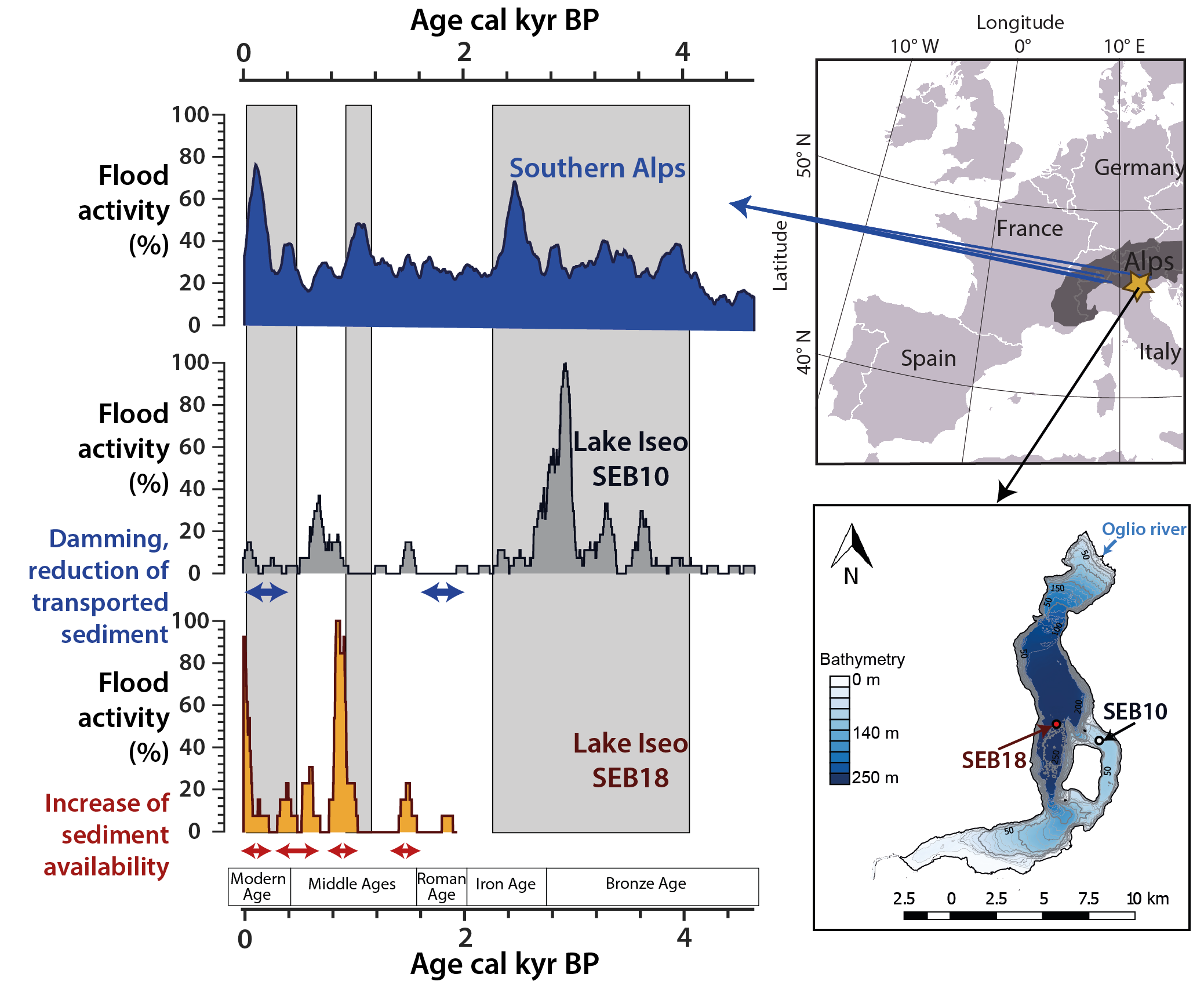
Figure 1: Flood activities modified from the Southern Alps synthesis of Wirth et al. (2013), the SEB10 (Rapuc et al. 2019) and SEB18 (unpublished) sediment sequences from Lake Iseo. Activity is calculated as a ratio of the instantaneous frequency and the maximum frequency measured in the sequence. Gray shading highlights periods of high regional flood frequency. |
Impact of human activities on erosion and transport processes
Sediment availability and transport processes are forced by both climatic fluctuations and human activities. Consequently, provided that the climatic conditions and methodologies of reconstruction are the same, discrepancies between flood chronicles in the same region should provide evidence of the influence of human activities. The Italian Southern Alps offer an ideal playground for such an experiment. Several lakes in this region have been studied and many flood chronicles have been produced; for example, Wirth et al. (2013) computed a Holocene synthesis of flood frequencies from five lake-sediment sequences from the Southern Alps.
Recently, we produced two flood chronicles from two sediment sequences taken from Lake Iseo, a large perialpine lake. The SEB18 sequence was sampled in the deep basin of the lake, fed by a large catchment (1777 km²). The SEB10 sequence (Rapuc et al. 2019) was retrieved in a shallower basin fed by sediment from a small catchment area (46.5 km²). The SEB10 flood chronicle is consistent with the regional extreme precipitation trend until the Roman Age (approx. 2 cal kyr BP), with an important increase in recorded flood frequency around 4.2 cal kyr BP, reflecting a shift towards wetter climate in Europe (Fig. 1; Wirth et al. 2013). However, the SEB10 sequence differs from the Southern Alps synthesis for periods when human activity is important in the Lake Iseo catchment (Fig. 1). For instance, during the Little Ice Age (LIA, 1300–1860 CE), flood activity in the Southern Alps was high due to a regionally colder and wetter climate, resulting in more frequent precipitation events. However, very few flood layers were deposited in the shallower basin of Lake Iseo at that time. We interpreted that discrepancy as resulting from the anthropization of the main tributaries (streams or rivers flowing into a larger stream or a main stem) through damming, thereby reducing sediment flux to the lake (Rapuc et al. 2019). At that study site, the creation of dams and channels in catchments generally deflected the river flow and trapped sediment upstream, hence reducing the sediment flux to the lake basin and the apparent flood frequency in the lake-sediment record.
 |
|
Figure 2: Conceptual model of the Critical Zone erosion cycle in a large catchment and the effects of the three main forcing factors: climate, geodynamics, and human activities. |
A different scenario was documented in SEB18. In this sequence, high flood frequencies are recorded during the Medieval Warm Period (950–1250 CE), and frequencies are lower than expected during the LIA (Fig. 1), in contrast to the regional trend (Wirth et al. 2013; Sabatier et al. 2017). Here, human activity is suspected to have impacted the erosion cycle in the catchment through grazing, agricultural activities, and deforestation, all of which lead to soil destabilization (Fig. 2). When soil erodibility increases and more sediment becomes available, the precipitation intensity necessary to entrain particles from the soil surface decreases (Renard et al. 1991). Hence, even a moderate precipitation event may be recorded as a graded layer in the lake basin, which artificially increases the flood frequency in the sediment record.
The comparison of the SEB10 and SEB18 sequences, taken from different sedimentary basins in the same lake, revealed different lake-sediment responses to the same climate forcing factors (Fig. 1). Moreover, the rise in flood frequency recorded in SEB10 during the High Middle Ages (1000–1250 CE) is delayed by 200 years compared to the SEB18 record. As all other factors are similar at these two core locations, only human-triggered changes in sediment availability or transport processes at the scale of catchment areas can explain these differences.
Summary and future work
Flood chronicles (frequencies and magnitudes) from lake sediments are robust paleoclimatic proxies in the absence of human activity modifying sediment availability in the catchment. However, when human activity affects the Critical Zone (CZ), defined as the reactive skin of our planet at the interface of lithosphere-atmosphere-hydrosphere-biosphere, by increasing erosion, resulting in increased sediment transport and remobilization, the sensitivity of a lake as a natural archive of the CZ dynamic is disturbed. A human-triggered increase in soil erodibility and sediment availability may therefore result in a decoupling of the recorded flood frequency and the regional climatic conditions. Inversely, stream management can result in a drastic decrease of river-borne sediment input. A similar phenomenon may result from other geodynamical processes, such as earthquakes (Rapuc et al. 2018): the sensitivity of a lake to record seismic shaking increases when sediment accumulation in the delta and on lake slopes increases (Fig. 2). To study paleohydrologic or geodynamic fluctuations, the safest way is then to investigate sediments retrieved from high altitude zones (Sabatier et al. 2017). However, large lakes draining large catchment areas offer us the opportunity to observe large-scale precipitation patterns. They are thus valuable resources for reconstructions of past flood frequency when considered together with the three main forcing factors driving erosion patterns and CZ dynamics throughout the Holocene: climate, geodynamics, and human activities (Fig. 2).
affiliation
Université Savoie Mont Blanc, Centre National de la Recherche Scientifique, Laboratoire Environnement, Dynamiques et Territoires de la Montagne, Le Bourget du lac, France
contact
William Rapuc: william.rapucuniv-smb.fr
references
Arnaud F et al. (2016) Quat Sci Rev 152: 1-18
Czymzik M et al. (2013) Quat Sci Rev 61: 96-110
Evin G et al. (2019) Glob Planet Change 172: 114-123
Glur L et al. (2013) Sci Rep 3: 2770
Rapuc W et al. (2018) Sedimentology 65: 1777-1799
Rapuc W et al. (2019) Glob Planet Change 175: 160-172
Rapuc W et al. (2020) Sediment Geol 409: 105776
Renard KG et al. (1991) J Soil Water Conserv 46: 30-33
Sabatier P et al. (2017) Quat Sci Rev 170: 121-135
Wilhelm B et al. (2018) Water Secur 3: 1-8
Peng Liang![]() , H. Li
, H. Li![]() , Y. Zhou, X. Fu
, Y. Zhou, X. Fu![]() , L. Mackenzie
, L. Mackenzie![]() and D. Zhang
and D. Zhang![]()
We analyze the recent progress in eolian surface processes and landscape dynamics in Chinese deserts. These diverse eolian studies, including paleoenvironmental reconstructions, advances in dating techniques, and clarification of sediment provenance, highlight the complexity of desert landscape evolution.
Drylands occupy ~41% of the global land surface and are home to more than two billion people (Reynolds et al. 2007). In recent decades, global warming and intensified human activities have exacerbated the environmental degradation or desertification in drylands, threatening nations' economies and sustainable development. Additionally, deserts are an important yet poorly understood component of the Earth system, with dust released from these regions affecting the global biogeochemical cycle and climate. Early-career researchers (ECRs) at Zhejiang University and elsewhere in China are currently investigating sedimentary archives from the interior of Chinese deserts in the eastern Asian desert belt (Fig. 1) to explore complex landscape dynamics through time.
 |
|
Figure 1: Distribution of Asian deserts, major rivers, and published data in the growing database. The thick dashed line indicates the boundary of the Asian summer monsoon. Active sand seas: Taklamakan (TK); Kumtagh (KT); Chaidamu (CD); Badain Jaran (BJ); Tengger (TG); Wulanbuhe (WB). Semi-stabilized sandy lands: Gurbantunggut (GT); Maowusu (MS); Kubuqi (KB); Hunshandake (HD); Horqin (HQ); Hulunbeier (HB). |
Paleoenvironmental signals archived in the eastern Chinese deserts
The large semi-stabilized sandy lands in the deserts of eastern China are located near the northern extent of the East Asian summer monsoon (Fig. 1). Stratigraphic sequences from the sandy lands record repeated periods of dune activation and stabilization through alternating eolian (wind-blown) sands and paleosols (buried soils). Dune stabilization processes are usually a landscape response to increased precipitation associated with enhanced summer monsoons, while increased eolian activity and dune activation occurs during periods of drought. These alternating sequences are a direct and sensitive record of past monsoon variability. Yang et al. (2019) found that a dark brown (Munsell soil color 10YR 4/3) paleosol began to develop at 14.5 thousand years before present (kyr BP) and lasted until 2 kyr BP in the Hulunbeier Sandy Land, while stronger pedogenesis (i.e. soil formation) occurred during 9-5 kyr BP. Eolian sequences from the Hunshandake Sandy Land recorded dune stabilization processes from 9.6 to 3.0 kyr BP, though localized eolian events occurred at the same time (Fig. 2). Although the paleolandscape in the eastern sandy lands shows a high degree of spatial heterogeneity, dunes were generally stabilized and eolian activity was suppressed from 7.5 to 3.5 kyr BP in the mid-Holocene (Fig. 2; Yang et al. 2019). These geological records from dune sequences are generally consistent with paleoclimate simulations, which indicate that northern China received higher summer monsoon precipitation during the mid-Holocene than during the pre-industrial period, although the moisture transport pathway is more complex in western Chinese deserts (Feng and Yang 2019).
 |
|
Figure 2: Eolian events represented by the frequency of optically stimulated luminescence (OSL) ages from the eastern sandy lands of northern China. The gray rectangles are OSL age histograms, and the bin size is 0.5 kyr. Data are from Li and Yang (2016) and Yang et al. (2019) with new data added. |
Spatial heterogeneity of the landscape leads to an unavoidable uncertainty when interpreting geological signals from eolian stratigraphic sequences. Liang and Yang (2016) investigated drivers of landscape heterogeneity at different scales in the Maowusu Sandy Land, northern China (Fig. 1). They found that climate and large-scale agricultural reclamation affect regional landscape patterns in the Maowusu Sandy Land, whereas microtopography and river networks drive landscape heterogeneity at a local scale. The landscape response to declining wind strength in the Maowusu Sandy Land from 1981 to 2016 shows a significantly out-of-step pattern between the western and eastern regions, arising from different regional climates and land-use histories (Liang and Yang 2016), highlighting the complexity of landscape dynamics in drylands.
The eolian processes at the dune scale also play an important role in the interpretation of paleoenvironmental records from dune deposits. The dune stabilization process is assumed to be mainly caused by precipitation-induced vegetation expansion. However, a new case study investigating the transition from barchan (crescent-shaped sand dune) to parabolic dunes in the Maowusu Sandy Land demonstrated that the reduction of wind strength can lower the sand flux rate and dune height, which allows for vegetation establishment and dune transformation (Zhang et al. 2020). This research suggests that some mismatches between dune activity and moisture variability could be reconciled through a better understanding of past wind regimes.
Improved dating techniques for paleoenvironmental reconstructions
Over the past 20 years, optically stimulated luminescence (OSL) dating has become a well-established Quaternary geochronometer, particularly for eolian sediments, and is arguably the most important tool for desert paleoenvironmental research. A series of luminescence dating procedures for K-feldspar, a ubiquitous mineral in natural sediments, has recently been developed using eolian and fluvial samples from Chinese deserts (Fu et al. 2015; Fu et al. 2018). These techniques considerably extend upper and lower dating limits and improve dating accuracy. The ability to analyze raw luminescence dating data has also been enhanced by a newly developed software "Luminescence Dose and Age Calculator (LDAC v1.0)" (Liang and Forman 2019; https://github.com/Peng-Liang/LDAC), which can maintain, archive, and synthesize basic OSL data, apply appropriate statistical models, calculate environmental dose rate, and render statistically significant final ages. This self-contained tool for luminescence dating allows for inter-laboratory OSL age comparisons and promotes more robust datasets for landscape-dynamics research in drylands and beyond. OSL dating of eolian sands has produced over 300 age records from dunes in China, which were recently compiled as part of the INQUA Dunes Atlas chronologic database (Li and Yang 2016; https://www.dri.edu/inquadunesatlas/). This primary dataset collated by ECRs has helped to build a picture of the eolian history in Chinese deserts since the Last Glacial Maximum, showing that the eolian events identified by the frequency of OSL ages increased during the last deglaciation and late Holocene but are mostly dormant during the mid-Holocene (Fig. 2). However, our understanding of eolian activity at the glacial-interglacial timescale is still unclear due to the lack of well-preserved and statistically meaningful archives older than 20 kyr BP from desert interiors, limiting regional multi-site paleoenvironmental reconstruction (Li and Yang 2016).
Sediment provenance and surface processes
Identifying sediment provenance can yield insights into understanding the complexity of past and present landscape dynamics in deserts. Sediment sources in the Taklamakan Desert, Badain Jaran Desert, Kubuqi Desert, and Maowusu Sandy Land were investigated by combining geochemical compositions of the sand with geomorphic analysis (Hu and Yang 2016; Liu and Yang 2018; Jiang and Yang 2019; Zhou et al. 2020). Results show that the dust fraction (<63 μm) in dune sands from the Taklamakan Desert varies from 0.44% to 21.7% and can be traced to the Kunlun and Tianshan Mountains by their geochemical and sedimentological characteristics. However, the sand particles (>63 μm) were predominantly sourced from the Kunlun Mountains in the south and transported via fluvial processes (Jiang and Yang 2019; Zhou et al. 2020). These results suggest that dust particles within deserts have independent provenance, which is consistent with the low dust-generation potential from sand saltation and wind abrasion found in wind-tunnel experiments (Adams and Soreghan 2020). Similarly, fluvial processes provide sand to the Badain Jaran Desert (Hu and Yang 2016), the Kubuqi Desert, and the Maowusu Sandy Land (Liu and Yang 2018) by transporting loose sediments from nearby mountains to the desert basins. These primary dune-building sediments are then further mixed via local eolian processes (Liu and Yang 2020).
Future work: moving to big data
The aforementioned case studies have greatly enriched our understanding of the landscape dynamics and surface processes in deserts of China and beyond, but a more comprehensive and continental-scale picture is still lacking. Paleoenvironmental reconstructions based on single-site dune deposits or sequences alternating between lacustrine, eolian sands, and paleosols in deserts inevitably contain uncertainties. These uncertainties mainly arise from the spatial heterogeneity of the eolian landscape (Liang and Yang 2016), the episodic/discontinuous eolian sand deposition features with possible eolian erosion (Forman 2015), and the generally non-linear response between eolian depositional processes and climate fluctuations (Yang et al. 2019). A big-data concept incorporating a continental-scale database using the substantial paleoenvironmental records from Chinese deserts could be introduced to overcome these difficulties and complexities. This database is currently under construction (Fig. 1) and will include sedimentary sequences that contain well-vetted geomorphic context information, stratigraphic descriptions, proxies (such as grain size, magnetic susceptibility), and relevant ages. A comprehensive and well-organized database that includes multiple physical and chemical indices of surface dune sand, such as grain size, geochemical composition, and petrology, is also required to advance sand provenance studies. These increasingly large and high-dimensional datasets and data-driven computations are a promising avenue to enhance our understanding of eolian processes and the Earth system from a big-data perspective, especially with the aid of machine learning algorithms. However, more in-depth field studies are still indispensable.
Acknowledgements
Our current work was supported mainly by the Ministry of Science & Technology of China (2017FY101001) and the National Natural Science Foundation of China (41672182; 42001003; 41430532). Sincere thanks are extended to the early-career researchers whose work we have cited, including Dr. Fangen Hu, Qianqian Liu, Qida Jiang and Yingying Feng. We also thank Dr. Ziting Liu and Wancang Zhao for enriching the ongoing database.
affiliation
School of Earth Sciences, Zhejiang University, Hangzhou, China
contact
Peng Liang: PLiangzju.edu.cn
references
Adams SM, Soreghan GS (2020) Geology 48: 1105-1109
Feng Y, Yang X (2019) J Geogr Sci 29: 2101-2121
Forman SL (2015) Front Earth Sci 3: 3
Fu X et al. (2015) Quat Geochronol 30: 161-167
Fu X et al. (2018) Quat Geochronol 47: 1-13
Hu F, Yang X (2016) Quat Sci Rev 131, Part A: 179-192
Jiang Q, Yang X (2019) J Geophys Res Earth Surf 124: 1217-1237
Li H, Yang X (2016) Quat Int 410: 58-68
Liang P, Forman SL (2019) Ancient TL 37: 21-40
Liang P, Yang X (2016) Catena 145: 321-333
Liu Q, Yang X (2018) Geomorphology 318: 354-374
Liu Q, Yang X (2020) J Desert Res 40: 158-168
Reynolds JF et al. (2007) Science 316: 847-851
Yang X et al. (2019) Sci China Earth Sci 62: 1302-1315
Zhang D et al. (2020) Earth Surf Process Landf 45: 2300-2313
Nitin Chaudhary![]()
The individual- and patch-based peatland-vegetation model LPJ-GUESS was employed to study past and future peatland carbon dynamics across the pan-Arctic. A substantial reduction in peatland sink capacity, expected under rapid global warming, has the potential to trigger important climate feedbacks.
Peatlands are important carbon reserves in the terrestrial ecosystem and cover 3% of the terrestrial land surface area (3.7 × 10⁶ km2; Bridgham et al. 2006, Hugelius et al. 2020). Peatlands store around 400–600 petagrams (1015 g) of carbon (PgC) since the Holocene and comprise around 30% of the present-day soil organic carbon pool (Yu et al. 2010; Hugelius et al. 2020). They are also a major source of atmospheric methane emissions (Abdalla et al. 2016). A significant fraction of peatland area coincides with permafrost, affecting carbon accumulation rates and biogeochemical processes (Obu et al. 2019). The majority of northern peatlands started developing 8000–12,000 years ago as a result of the availability of new land surface following deglaciation, warmer climate conditions, higher summer insolation, more pronounced seasonality, elevated greenhouse gas emissions, and higher moisture conditions (MacDonald et al. 2006). However, present-day distribution of soil organic carbon is not uniform across the pan-Arctic region (45–75°N) due to differential peat initiation periods, bulk density values, and changes in dominant plant types (Loisel et al. 2014). Recent advances in field measurements have reduced some uncertainties related to carbon accumulation rates and peat depth across the pan-Arctic (Loisel et al. 2014). However, due to the large extent of peatlands, calculating global and regional estimates directly from field measurements would be difficult. This difficulty can be circumvented by employing peatland models, as these simulate realistic peatland carbon accumulation rates at larger spatial and temporal scales and can further strengthen the recent progress on observing carbon accumulation rates (Stocker et al. 2014; Chaudhary et al. 2017a, b). Understanding long-term peatland carbon dynamics and their controls are crucial for predicting their role in moderating future climate.
Dynamic peatland-vegetation models and long-term carbon dynamics
Dynamic global vegetation models (DGVMs) such as LPJ-GUESS (Lund-Potsdam-Jena General Ecosystem Simulator) are used to understand the changes in vegetation, carbon cycle, and climate feedbacks on different temporal and spatial scales. They provide a suitable platform to study long-term peatland carbon dynamics, enabling us to understand the role of peatlands in past and future climate conditions. To this end, a recent study demonstrated a new implementation of peatland and permafrost dynamics with the unique representation of spatial heterogeneity in the dynamic global vegetation model (in LPJ-GUESS; Chaudhary et al. 2017a). This was the first time that any model included dynamic annual multi-layer peat accumulation, freezing-thawing cycles, lateral flow, and spatial heterogeneity in the framework of a dynamic vegetation model (Chaudhary et al. 2017a), and was applied at local to regional spatial scales.
The current model scheme consists of many key variables and interactions controlling the non-linear peatland dynamics (Chaudhary et al. 2018). The relationship between the average rate of peat formation and water table position (Belyea 2009), cyclicity among micro-formations (hummocks and hollows) (Heikki 2002), internal eco-hydrological feedbacks, and multi-directionality (Belyea 2009) that have frequently been observed in many peatland sites can be simulated and explained using this detailed model scheme. The model has been applied in different regions in the Northern Hemisphere and shown to reproduce peat accumulation, permafrost dynamics, and vegetation distribution realistically in several Scandinavian sites (Chaudhary et al. 2017a).
 |
|
Figure 1: Modeled net peatland carbon accumulation rates (in gC m2/yr) across the pan-Arctic (A) at present (1991–2000) and (B) at the end of the century (2091–2100). Positive values indicate carbon sinks, and negative values represent sources of carbon from peatlands to the atmosphere (Chaudhary et al. 2020). |
Changes in peatland carbon stocks in the future
Peatlands are severely threatened by ongoing anthropogenic climate warming, and it is expected that many peatland regions will experience significant changes in their carbon fluxes in the near future. Subsequent regional (pan-Arctic) studies employing the model described above (Chaudhary et al. 2017b; 2020) found that many peatland regions in Europe, including Scandinavia and Russia, and central and eastern Canada would change from carbon sinks to potential carbon sources in the coming century, while other sites would enhance their sink capacity at other sites (Fig. 1). It was found that permafrost peatlands are likely to accumulate more peat in warmer conditions due to the high level of moisture that results from permafrost thaw, higher precipitation, and elevated CO2 levels. On the other hand, peatlands that experience reduced precipitation rates and are devoid of underlying permafrost will lose more carbon in the future, particularly peatlands located in the European region and peatlands between 45° and 55°N. Overall, the study showed that peatlands would continue to act as carbon sinks, but their sink capacity will be substantially reduced under rapid global warming (Fig. 1b) in the coming decades.
Peatland-mediated feedbacks
The rapid, ongoing changes in many peatland areas due to climate change have the potential to disturb the prevailing land-atmosphere carbon balance and trigger some pertinent climate-relevant feedbacks. The higher carbon emissions from peatlands as a result of climate warming could result in a positive feedback on climate change, thus amplifying warming (Baird et al. 2009; Frolking et al. 2009). On the other hand, elevated CO2 concentrations in the atmosphere together with an increase in moisture conditions due to permafrost thawing and higher precipitation rates could promote plant growth and peat accumulation (Loisel and Yu 2013). This, in turn, may enhance the carbon (i.e. CO2) uptake capacity of many peatlands and would be expected to result in a negative feedback on climate warming. In addition, an increase in the active layer depth or soil moisture due to temperature-driven permafrost degradation and structural collapse of many peatland sites located in cold environments could lead to the formation of wet and water-filled areas (Belyea 2009; Turetsky et al. 2019). This would most likely result in higher methane emissions that would further accelerate regional warming. However, the net effect of all these competing peatland-mediated feedbacks is difficult to study in isolation. For that, an integrated study is required that takes all the critical interactions and feedbacks between peatland carbon cycle and climate into account.
 |
|
Figure 2: A proposed schematic representation of the regional Earth system model RCA-GUESS. |
Integrating peatland dynamics in Earth system models
Contemporary Earth system models simulate the state of the atmosphere and biosphere at different spatial and temporal scales and predict their responses and behavior in rapidly changing climate conditions. However, these advanced models currently lack peatlands as a distinct land surface type (Frolking et al. 2009). Due to the absence of a comprehensive representation of detailed peatland and cryospheric processes in any of the current Earth system models, our understanding of these hypothesized peatland-mediated feedbacks on regional and global scales is limited. The peatland dynamics in LPJ-GUESS seem to be reasonable, as the model produces realistic carbon accumulation rates and permafrost distribution at different spatial and temporal scales (Chaudhary et al. 2020). With this peatland extension, the coupled regional Earth system model (RCA-GUESS) will be appropriate for addressing questions related to short-term and long-term effects of peatland dynamics on regional climate (Fig. 2). The model will be employed in the pan-Arctic region to quantify the magnitude, direction, and strengths of peatland carbon-climate feedbacks; these results will then be fed into the land-surface module of the global Earth system model to improve global peatland modeling.
affiliations
Department of Physical Geography and Ecosystem Science, Lund University, Sweden
Department of Geosciences, University of Oslo, Norway
contact
Nitin Chaudhary: nitin.chaudharynateko.lu.se, nitin.chjgmail.com
references
Abdalla M et al. (2016) Ecol Evol 6: 7080-7102
Bridgham SD et al. (2006) Wetlands 26: 889-916
Chaudhary N et al. (2017a) Biogeosciences 14: 2571-2596
Chaudhary N et al. (2017b) Biogeosciences 14: 4023-4044
Chaudhary N et al. (2018) Ecosystems 21: 1196-1214
Chaudhary N et al. (2020) Global Change Biol 26: 4119-4133
Heikki S (2002) Fennia Int J Geogr 180: 43-60
Hugelius G et al. (2020) Proc Natl Acad Sci USA 117: 20438-20446
Loisel J, Yu Z (2013) J Geophys Res Biogeosci 118: 41-53
Loisel J et al. (2014) Holocene 24: 1028-1042
MacDonald GM et al. (2006) Science 314: 285-288
Obu J et al. (2019) Earth-Sci Rev 193: 299-316
Stocker BD et al. (2014) Geosci Model Dev 7: 3089-3110
Amy C.F. King![]() 1 and Dieter R. Tetzner
1 and Dieter R. Tetzner![]() 1,2
1,2
New ice-core records are being developed from the sub-Antarctic, a region previously lacking in paleoclimate archives. These records capture marine-sourced organic compounds that act as proxies for sea-ice concentration, and wind-lofted diatoms that reflect westerly wind strength.
The sub-Antarctic region is critical to our understanding of past changes in westerly wind strength, sea-ice extent, Southern Ocean biogeochemical cycling, and processes interfacing polar and mid-latitude climate. Yet this region, defined here as southward of the Southern Ocean polar front, is severely lacking in paleoclimate archives. Consequently, our ability to predict future changes in these processes is limited. To answer the need for new climate records, the 2016–2017 Antarctic Circumnavigation Expedition (https://spi-ace-expedition.ch/) collected a suite of shallow (12–24 m depth) ice cores from ice-capped islands and glaciers throughout the Antarctic and sub-Antarctic (Fig. 1). The cores are climate archives for the late 20th century to present day (Thomas et al. 2020). Due to the logistical challenges of accessing such remote islands, several of these cores are the first to have ever been drilled at these sites.
 |
|
Figure 1: Locations of new sub-Antarctic ice cores (squares), alongside locations of cores previously used for reconstructing sea ice (yellow circles) and westerly winds (yellow/red circle) for the last 2000 years. Winter (WSIE) and summer sea-ice extent (SSIE; source: https://nsidc.org/data/g02135) are included for reference. |
The main objective of the sub-Antarctic ice-core drilling expedition is to "plug the gap" by providing paleoclimate records from the data-sparse sub-Antarctic. The PAGES2k Consortium (2017) highlighted the absence of paleoclimate archives across the Southern Ocean. Their global composite database of 692 temperature-sensitive records from 648 locations provides no spatial coverage in the sub-Antarctic. Improving spatial fidelity of records is another project goal. Ice-core reconstructions of marine-sourced components so far rely on cores from coastal Antarctica. Source regions of marine compounds found in these cores may cover entire ocean sectors (shown in Fig. 1). This means local-scale past climatic changes are not captured.
Alongside the collection of new cores has been the development of a number of novel ice-core proxies, focussing on emissions from the marine biosphere. Sub-Antarctic islands are in areas of marine productivity, therefore sub-Antarctic cores ideally lend themselves to marine-sourced proxies. This article highlights the exciting potential of these new proxies for sea-ice concentration and westerly wind strength, both key drivers in global climate dynamics.
Diatoms as proxies for westerly winds
Diatoms are unicellular algae with siliceous cell walls, found in surface waters worldwide. They are especially abundant in major oceanic water-mass convergence zones, such as the Southern Ocean, where nutrient upwelling leads to high productivity. Diatoms are lifted from the ocean surface into the atmosphere by wind-induced bubble-bursting and wave-breaking processes (Cipriano and Blanchard 1981; Farmer et al. 1993). Once in the atmosphere, they can be transported by strong winds over long distances. In polar regions, airborne diatoms are deposited over ice sheets and ice caps, and incorporated into the ice-core record (Budgeon et al. 2012).
Marine and non-marine diatoms have been found in ice cores from several locations across Antarctica (Kellogg and Kellogg 2005). Diatoms are found throughout the Southern Ocean, but Pike et al. (2008) observed the largest blooms occurred during spring near the Antarctic Polar Front zone, the sea-ice margin, or both. In light of this, Allen et al. (2020) and Tetzner et al. (2021) explored the abundance and diversity of diatoms preserved in Antarctic ice cores, highlighting their potential as proxies of wind strength and atmospheric circulation in the Southern Ocean.
 |
|
Figure 2: Location of Bouvet with geographical areas where core compound concentrations positively correlate with sea-ice concentration (R = 0.6, p < 5%), and area where diatom concentration correlates with westerly winds (R = 0.6, p < 5%). Also shown, how these correspond to winter (WSIE) and summer sea-ice extent (SSIE), and the Antarctic Polar Front (APF). |
The Peter 1st and Bouvet ice cores (providing climate records for 1999–2017 and 2001–2017, respectively) were obtained from two strategic locations to track changes in the westerly wind belt. Preliminary results from Tetzner et al. (2021), indicate that the Peter 1st ice-core diatom record presents correlations with winds in several locations; a positive correlation (R > 0.8, p < 5%) with ERA5-reanalysis wind strength in the westerly wind belt north of the Amundsen-Bellingshausen Sea, a positive (negative) correlation with latitudinal winds over the westerly wind belt (Antarctic coastal easterlies), and a positive correlation with offshore winds over the Amundsen Sea. These evidence the imprint of the Amundsen Sea low-pressure center driving the regional atmospheric circulation. Similarly, preliminary results from the Bouvet ice-core diatom record show a positive correlation (R > 0.7, p < 5%) with wind strength over the westerly wind belt (Fig. 2). This is supported by a positive (negative) correlation with latitudinal winds over the westerly wind belt (Antarctic coastal easterlies) and a positive (negative) correlation with offshore (onshore) winds over the Weddell Sea. Both indicate that the presence of the Weddell low-pressure center drives the regional atmospheric circulation.
Preliminary results from these ice cores highlight their diatom records as valuable proxies of regional wind strength and atmospheric circulation in the sub-Antarctic region.
Novel organic compounds as sea-ice markers
Organic compounds are emitted from the surface ocean into the atmosphere by biochemical and physical processes. They are infrequently investigated in Antarctic ice-core records due to low concentrations, a lack of current understanding, or both. One established marine organic proxy is methanesulfonic acid (MSA). MSA is an oxidation product of dimethyl sulfide, a chemical compound produced by phytoplankton blooms containing diatoms. Curran and Jones (2000) first proposed that MSA concentration may be interpreted as a sea-ice proxy under the following mechanisms: (1) Antarctic winters with a greater sea-ice extent also have a larger area of sea-ice decay during the following spring melt; (2) This bigger sea-ice break-up zone enhances phytoplankton blooming, and subsequently, production of MSA; (3) Atmospheric transport deposits MSA onto ice caps, incorporating the varying yearly concentrations into ice-core records.
Giorio et al. (2018) discussed a wealth of additional marine organic compounds that show potential for use as paleoclimate indicators. Analytical advances developed by King et al. (2019a), provided a method for analyzing up to 30 of these novel compounds simultaneously in ice samples. King et al. (2019b) subsequently applied these methods, alongside MSA analysis, to the first ever ice core drilled on the sub-Antarctic island Bouvet.
Results of the Bouvet ice-core analyses show a positive correlation (R = 0.79; p < 1%) between annual concentrations of MSA and oleic acid, the latter a fatty acid found in diatoms. Further investigation shows that a direct, positive correlation between annual oleic acid concentrations and each year's winter sea-ice concentration is found in a geographical area extending west of Bouvet Island, tracing the margin of maximum winter sea-ice extent (Fig. 2). Back-trajectory analysis (King et al. 2019b) ties the story together: westerly winds transport MSA and oleic acid, from spring blooming events in the sea-ice break-up zone to the west of Bouvet Island to the ice-core site, where they are deposited. Greater concentrations of MSA and oleic acid are emitted, transported, and deposited in years of greater maximum winter sea-ice extent.
The Bouvet ice-core analyses have also produced records of the marine organic compounds oxalate, formate, and acetate. Compound concentrations positively correlate with sea-ice concentration (King et al. 2019b). In contrast to oleic acid and MSA, the correlation exists for summer sea-ice concentration in a region south of Bouvet Island (Fig. 2). A better understanding of the sources of these compounds is required to definitely define the mechanism behind this correlation.
Analysis of the Bouvet core shows great promise for the development of a suite of marine organic sea-ice markers in sub-Antarctic ice cores.
Future directions
Investigation of novel marine-sourced components in ice cores presents new climate proxies in the sub-Antarctic over the past few decades. Organic compound concentrations record variations in sea-ice concentration, and diatoms record westerly wind strength. Thus, diatoms and the fatty acid compounds they produce commonly link records of both emissions and transport of these components. Future work analyzing these components in further sub-Antarctic island cores will allow us to develop these archives throughout the sub-Antarctic, and extend records further back in time. Combining sea-ice proxy records from both marine-sediment and ice cores (Thomas et al. 2019) may provide sea-ice paleorecords of improved accuracy, longevity, and spatial coverage. All of these factors provide the critical context needed for improving future projections of change in the climate-influencing sub-Antarctic region.
Acknowledgements
Many thanks to Claire S. Allen for producing the Southern Ocean bathymetry map.
affiliations
1British Antarctic Survey, Cambridge, UK
2Department of Earth Sciences, University of Cambridge, UK
contact
Amy King: amykingbas.ac.uk
references
Allen CS et al. (2020) Geosciences 10: 87
Budgeon A et al. (2012) Antarct Sci 24: 527-535
Cipriano RJ, Blanchard D C (1981) J Geophys Res 86: 8085–8092
Curran MAJ, Jones B (2000) J Geophys Res Atmos 105: 451–459
Farmer D et al. (1993) Nature 361: 620–623
Giorio C et al. (2018) Quat Sci Rev 183: 1-22
Kellogg D, Kellogg T (2005) In: Castello J, Rogers S (Eds), Life in Ancient Ice. Princeton University Press, 69-93
King ACF et al. (2019a) Talanta 194: 233–242
King ACF et al. (2019b) Geophys Res Lett 46: 9930–9939
PAGES2k Consortium (2017) Sci Data 11: 1–33
Pike J et al. (2008) Mar Micropaleontol 67(3-4): 274-287
Tetzner D et al. (2021) Front Earth Sci 9: 617043
Thomas ER et al. (2019) Geosciences 9(12): 506
Thomas ER et al. (2020) Cryosphere Discuss, doi:10.5194/tc-2020-110
Georgia R. Grant![]() 1 and Tim R. Naish
1 and Tim R. Naish![]() 2
2
We reassess available studies of mid-Pliocene sea level and provide new estimates. The relative amplitude of glacial-interglacial sea-level variability was likely between 6.2 m (16th percentile) and 16.7 m (84th percentile), leading to an average ice-volume sensitivity of 4 m/°C sea-level equivalent.
The mid-Pliocene warm period (MPWP), 3.3–3 million years ago, is the most recent time when Earth's climate reached equilibrium under atmospheric CO2 concentration of ~400 ppm, with global temperatures 2–3°C higher than during the pre-industrial era (1750 CE; Masson-Delmotte et al. 2013). Sea-level reconstructions for this period suggest peak interglacial sea levels were up to 40 m above present (e.g. Dutton et al. 2015), implying loss of the Greenland, West Antarctic, and marine sectors of the East Antarctic ice sheets, as well as partial loss of the terrestrial East Antarctic Ice Sheet.
Peak magnitude vs relative amplitude
Reconstructions of peak MPWP interglacial sea level are usually reported as global mean sea level (GMSL) with reference to the Holocene. While peak GMSL provides insight into the volume of polar ice-sheet loss and the magnitude of sea-level rise that might be expected because of near-future climate change, it does not capture the full amplitude of glacial-interglacial ice-volume change (Fig. 1), or the full amplitude of sea-level change in response to climate forcing, which may lead to an underestimation of ice volume sensitivity (defined here as the change in sea level equivalent (SLE) of ice volume (m) per 1°C of temperature change). For example, calibrations of the benthic δ18O proxy of global ice volume and sea level (e.g. Lisiecki and Raymo 2005) place the sea level during many Pliocene glacials below that of present-day, implying larger-than-present ice-sheet configurations at the beginning of deglaciations. This has significant implications for estimating both the amplitude and rate of sea-level rise in response to relatively small amounts of global warming.
 |
|
Figure 1: Studies of MPWP sea-level estimates (shown in Fig. 2) are placed into four categories. The schematic sea-level curve illustrates the difference between peak GMSL as a single point referenced to a datum, and relative amplitude of sea-level change over the glacial-interglacial range. |
We have categorized "continuous" sedimentary sequences used in reconstructing the amplitude of MPWP GMSL into "direct" (e.g. geologic) and "indirect" (e.g. calibrations of foraminifera δ18O curves; Fig. 1; Fig. 2a). We compare these glacial-interglacial amplitudes with estimates of the peak MPWP GMSL derived from "direct" but "discontinuous" geological remnants preserved in the far field (e.g. paleo shorelines). In addition, we use ice-volume constraints provided by polar continental margin drill cores (Fig. 1; Fig. 2b). Finally, we provide a quantitative reassessment of peak GMSL and the amplitude of glacial-interglacial global sea-level change during MPWP.
Where the uncertainty lies
Many of these peak GMSL estimates have not been corrected for regional deviations due to tectonics, glacio-isostatic adjustment (GIA), or dynamic topography. Deformation of the Earth may cause local sea-level changes large enough to either cancel out or double the amplitude of the ice-volume contribution (Raymo et al. 2011). Although some recent studies have attempted to correct for these regional effects, significant uncertainty remains concerning the role of dynamic topography (Rovere et al. 2015; Dumitru et al. 2019).
Deep-ocean foraminiferal δ18O records provide one of the most detailed proxies for glacial-interglacial climate variability during the Pliocene; however, the signal is affected by ocean temperature, ice-sheet δ18O composition and ice volume (Lisiecki and Raymo 2005). Several studies have used Mg/Ca paleothermometry to calibrate benthic δ18O records (Dwyer and Chandler 2009; Sosdian and Rosenthal 2009; Miller et al. 2012; Miller et al. 2020). Another approach incorporates sill-depth and salinity changes from the Mediterranean to calibrate sea level in a planktic δ18O record (Rohling et al. 2014), but large uncertainties (>±10 m) remain. On the other hand, sea-level calibrations of the benthic δ18O record, constrained by backstripped continental margins (sedimentary sequences that have tectonic subsidence and compaction effects removed; e.g. Naish and Wilson 2009; Miller et al. 2012; Miller et al. 2020), are often hampered by the limited precision inherent to foraminiferal paleodepth indicators and the influence of sediment erosion during sea-level low-stands, leading to underestimation of the full amplitude of sea-level change.
 |
|
Figure 2: (A) Frequency distributions of relative sea-level amplitudes for continuous studies of the MPWP with box and whisker plots for the 10th, 16th, 50th, 84th, and 90th percentiles with cumulative sea-level equivalent shown for marine-based ice sheets (MBIS) of Antarctic Ice Sheets (AIS), Greenland Ice Sheet (GIS) and terrestrial AIS; and (B) PlioSeaNZ relative amplitude percentiles shown as horizontal colored bars in comparison to peak GMSL estimates and geologic constraints on ice-sheet contribution to sea level. An R script and R workspace for these plots are available on request from the author. Note that Study 2 only spans part of the MPWP. |
In contrast, Grant et al. (2019) derived a continuous but floating sea-level record for the MPWP termed PlioSeaNZ from Whanganui, New Zealand, that is completely independent of the global benthic δ18O record. It calculates a theoretical relationship between sediment transport by waves and water depth, and applies the technique to grain size in a well-dated, continuous, shallow marine sequence. Water-depth variations obtained in this way, after corrections for compaction, tectonic subsidence, and glacial isostatic adjustment (GIA), yield the full amplitude of glacial-interglacial sea-level variability with precision of ±5 m and are relatively unaffected by dynamic topography.
Revisited estimates
The amplitude of glacial-to-interglacial sea-level change in continuous sedimentary records spanning MPWP (Fig. 1 and references therein) are compared in Figure 2a. The relative amplitude (maximum range) is calculated for a moving 20,000-year window at variable time steps for each record determined by sample spacing in the individual records. The 20,000-year window is chosen to capture the minimum orbital frequency of change. Also plotted are the percentiles (10th, 16th, 50th, 84th, 90th) for the amplitude-frequency distributions.
If these amplitudes are treated as GMSL change above present and the current global ice-sheet budget is considered the potential meltwater source, the sea-level equivalent of marine-based portions (MBIS) of the Antarctic Ice Sheet can account for 22.7 m, the Greenland Ice Sheet contains 7.3 m, and an additional 35.6 m is available from terrestrial sectors of the Antarctic Ice Sheet. Amplitudes >+30 m can only be explained by melting the terrestrial sectors of the Antarctic Ice Sheet, and/or by having more ice on the Northern Hemisphere continents during glacial periods than can be explained by the available geological data (e.g. Thiede et al. 2011). Larger-than-Holocene Antarctic glacial ice volumes cannot be excluded by proximal geological data for every glacial of the MPWP (Naish et al. 2009), but retreat of the East Antarctic Ice Sheet since eight million years ago is precluded by a recent study that found extremely low concentrations of cosmogenic 10Be and 26Al isotopes in the ANDRILL-1B marine sediment core (Shakun et al. 2018).
If all the variability in the PlioSeaNZ record was above present-day sea level, then GMSL during the warmest mid-Pliocene interglacial was at least +4.1 m and no more than +20.7 m, with a median of +10.7 m and likely (66%) range between 6.2 m (16th percentile) and 16.7 m (84th percentile; Fig. 2b). This maximum range is consistent with sediment composition from polar continental sediment cores, far-field sea-level reconstructions (Fig. 2b and refs. therein), and ice-sheet model constraints (e.g. DeConto and Pollard 2016). On this basis, we suggest that estimates using a calibration of the deep-sea δ18O record by Mg/Ca paleothermometry and a sill depth-salinity relationship tend to overestimate the amplitude of global sea-level change during the MPWP.
This range also implies an equilibrium polar ice-sheet sensitivity of 2–8 m of sea-level change for every degree of temperature change, with a mean value of 4 m/°C. This empirical estimate does not consider ice-sheet dynamics, such as a potential stability threshold in the Antarctic Ice Sheet, caused by the loss of ice shelves, which may be crossed at 1.5–2°C of global warming, after which ongoing mass loss may be rapid and non-linear (Golledge et al. 2015).
affiliations
1Department of Surface Geosciences, GNS Science, Lower Hutt, New Zealand
2Antarctic Research Centre, Victoria University of Wellington, New Zealand
contact
Georgia Grant: G.Grantgns.cri.nz
references
DeConto RM, Pollard D (2016) Nature 531: 591-597
Dumitru OA et al. (2019) Nature 574: 233–236
Dutton A et al. (2015) Science 349: aaa4019
Dwyer GS, Chandler MA (2009) Philos Trans Royal Soc A 367: 157-168
Golledge NR et al. (2015) Nature 526: 421-425
Grant GR et al. (2019) Nature 574: 237-24
Lisiecki LE, Raymo ME (2005) Paleoceanography 20: PA1003
Miller KG et al. (2012) Geology 40: 407-410
Miller KG et al. (2020) Science 6: eaaz1346
Naish TR et al. (2009) Nature 458: 322-328
Naish TR, Wilson GS (2009) Philos Trans Royal Soc A 367: 169-87
Raymo ME et al. (2011) Nature Geosci 4: 328-332
Rohling EJ et al. (2014) Nature 508: 477-482
Rovere A et al. (2015) Earth Sci Rev 145: 117-131
Shakun JD et al. (2018) Nature 558: 284-287