PAGES Magazine articles

Nathaelle Bouttes¹, F. Lhardy¹, D.M. Roche^1,2 and T. Mandonnet¹

Past carbon cycle changes, especially during the Last Glacial Maximum 21,000 years ago, remain largely unexplained and difficult to simulate with numerical models. The ongoing PMIP-carbon project compares results from different models to improve our understanding of carbon cycle modeling.

PMIP-carbon

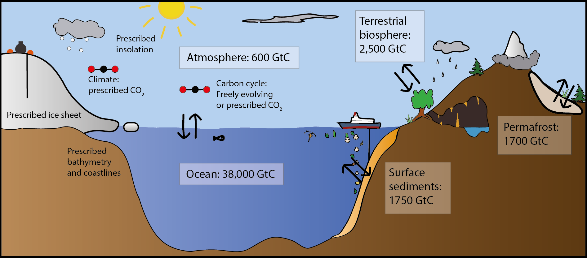
Atmospheric CO₂ concentration plays a major role for the Earth's climate as this is one of the main greenhouse gases. Moreover, the CO₂ level directly influences the ocean pH with large impacts on marine biology. Hence, understanding the carbon cycle, and its past changes, is critical. The carbon cycle at short timescales corresponds to the exchange of carbon between the main carbon reservoirs: ocean, atmosphere, terrestrial biosphere, surface sediments, and permafrost (Fig. 1). The atmospheric CO₂ concentration depends on the carbon fluxes and how much carbon is stored in the various reservoirs.

Figure 1: Schematic of the short-term carbon cycle with the main reservoirs and their estimated carbon content at the pre-industrial. The long-term processes (longer than 100 kyr) such as volcanism or silicate weathering are not considered. Also indicated are the boundary conditions imposed in climate models and the two types of simulation of atmospheric CO2.

We know from proxy data that the atmospheric CO₂ level has varied largely in the past. In particular, measurements of CO₂ concentration in air bubbles trapped in ice cores indicate lower values of ∼190 ppm during cold glacial periods compared to values of ∼280 ppm during warmer interglacial periods (Bereiter et al. 2015 and references therein). Many studies have focused on explaining the low CO₂ during the Last Glacial Maximum (LGM), but no consensus on the main mechanisms has been reached yet. Most models do not simulate such a low value, especially when they are simultaneously constrained by other proxy data such as carbon isotope values.

Nonetheless, several potential mechanisms have emerged (Bouttes et al. 2021). Firstly, the ocean is assumed to play a major role; this is the largest reservoir relevant for these timescales, meaning that any small change in its carbon storage could result in large modifications in the atmospheric CO₂ concentration. In addition, proxy data, such as carbon isotopes, seem to indicate changes in ocean dynamics and/or biological production. Besides the ocean, the sediment and permafrost reservoirs have also expanded during the LGM, helping to decrease atmospheric CO₂. Conversely, the terrestrial biosphere lost carbon at the LGM, indicating that even more carbon was taken up by the other reservoirs.

Until now, the different working groups within PMIP have mainly focused on climate without considering carbon cycle changes. A new project was recently defined as part of the deglacial working group in PMIP4 to tackle the issue of past carbon cycle changes. The objectives of this model intercomparison are to evaluate model responses in order to better understand the changes, help find the major mechanisms responsible for the carbon cycle changes, and improve models. As a starting point, the project focuses on the LGM, hence the protocol follows the main LGM PMIP4 guidelines for greenhouse gases, insolation, and ice sheets, as closely as possible (Kageyama et al. 2017). The same numerical code should be used for the pre-industrial period and the LGM, including the carbon cycle modules.

First results: Carbon storage changes in the main three reservoirs

So far, three GCMs (MIROC-ES2L, CESM and IPSL-CM5A2), four EMICs (CLIMBER-2, iLOVECLIM, MIROC-ES2L, LOVECLIM, UVic), and one ocean only GCM (MIROC4m) have been participating in PMIP-carbon. As not all models have all carbon cycle components (particularly sediments and permafrost), this first intercomparison exercise is focused on simulations with the ocean, terrestrial biosphere, and atmosphere carbon reservoirs only.

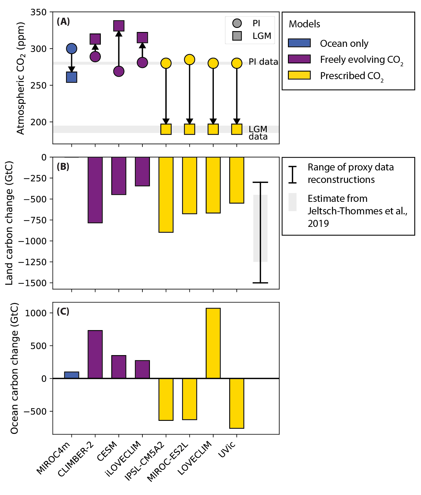
It should be noted that there are often two CO₂ variables in models: one for the radiative code—generally fixed to a prescribed value to ensure a correct climate—and another one for the carbon cycle. The latter can be prescribed to the same values as the CO₂ for the radiative code (yellow in Fig. 2a) or can be allowed to evolve freely in the carbon cycle model based on the fluxes with the other carbon reservoirs (purple and blue in Fig. 2a).

The most striking result is that in models that do not prescribe atmospheric CO₂ and include the terrestrial biosphere (purple in Fig. 2a), the LGM CO₂ concentration is higher than during the pre-industrial, rather than lower, as indicated by the data. In the ocean-only model (blue in Fig. 2a), the CO₂ is lower at the LGM, but the amplitude is very small compared to the data.

Figure 2: Carbon in three reservoirs: (A) Atmospheric CO2 concentration (ppm), (B) terrestrial biosphere carbon change from PI to LGM (GtC) and (C) ocean carbon change (GtC). CO2 data from Bereiter et al. (2015). Reconstruction of terrestrial biosphere carbon change using proxy data ranging from 300 GtC with carbon isotopes to 1500 GtC from pollen records (see Jeltsch-Thommes et al. 2019 for a more in-depth discussion).

In agreement with data reconstructions, the land carbon storage (vegetation and soils) decreases from the pre-industrial to the LGM (Fig. 2b) due to the colder LGM climate and larger ice sheets. The amplitude of this decrease varies between models, possibly due to differences in the terrestrial biosphere modules, and differences in the simulated climate (Kageyama et al. 2021). However, this could also result from different prescribed boundary conditions, such as coastlines and ice-sheet extents, both of which yield different land surfaces at the LGM and, hence, more or less space for vegetation to grow.

In the ocean, model results are more variable. Most models with prescribed atmospheric CO₂ (except LOVECLIM) indicate a loss of ocean carbon storage, at odds with the general view of increased carbon storage. In the models with freely evolving CO₂, the ocean stores more carbon (a similar result is seen in LOVECLIM simulations), but this effect is far too small to counteract the loss of carbon from land. This, therefore, results in atmospheric CO₂ values far outside of the range of the data.

The carbon storage in the ocean is the result of many competing processes. For example, on the one hand, lower temperatures increase CO₂ solubility, and increased nutrient concentrations due to lower sea level (of ∼130 m) yields more productivity, both lowering atmospheric CO₂. On the other hand, the increased salinity due to sea-level change tends to increase atmospheric CO₂. While these mechanisms are relatively well understood, the change of ocean circulation is still a major issue in models (Kageyama et al. 2021). PMIP-carbon aims to understand these model differences and highlight missing processes in the ocean.

One result that has already emerged is the importance of the ocean volume: at the LGM the ocean volume was reduced by ∼3% due to the sea-level drop, yielding a reduced ocean carbon reservoir size (Lhardy et al. 2021). This means that the ocean (by means of other processes), sediments, and permafrost have to store even more carbon to counteract this effect. For modeling groups, it also means that accounting for realistic bathymetry and coastline changes is essential; at the very least, the changes of oceanic variable concentrations such as alkalinity in models must be treated with great care.

Looking forward

In the short-term, PMIP-carbon will aim for more in-depth analyses of the ocean and terrestrial biosphere to understand the differences between models using existing (and ongoing) simulations.

However, the atmospheric CO₂ change that has to be explained is actually more than just the observed 90 ppm fall. Several changes tend to increase the CO₂ concentration, such as the loss of terrestrial biosphere, or the reduced ocean volume due to lower sea level. Hence, in addition to oceanic processes, other carbon reservoirs, such as sediments and permafrost, will be essential to explain the lower atmospheric CO₂. In the future, these additional components will be added to the protocol and their effects will be compared between models.

Finally, even if the LGM is an interesting period to study, the long-term objective of PMIP-carbon is to also compare model results during other periods such as the last deglaciation for which more challenges will arise: on top of the large glacial-interglacial 90 ppm change, the transition shows rapid changes in the carbon cycle which are not yet well understood (Marcott et al. 2014).

Affiliations

¹Laboratoire des Sciences du Climat et de l'Environnement, LSCE/IPSL, UMR CEA-CNRS-UVSQ, Université Paris-Saclay, Gif sur Yvette, France

²Faculty of Science, Department of Earth Sciences, Vrije Universiteit Amsterdam, The Netherlands

contact

Nathaelle Bouttes: nathaelle.boutteslsce.ipsl.fr

references

Bereiter B et al. (2015) Geophys Res Lett 42: 542-549

Bouttes N et al. (2021) In: Ramstein G et al. (Eds) Paleoclimatology. Frontiers in Earth Sciences. Springer, 271-300

Jeltsch-Thömmes A et al. (2019) Clim Past 15: 849-879

Kageyama M et al. (2017) Geosci Model Dev 10: 4035-4055

Kageyama M et al. (2021) Clim Past 17: 1065-1089

Lhardy F et al. (2021) Paleoceanogr Paleoclimatol 36: e2021PA004302

Marcott S et al. (2014) Nature 514: 616-619

Fabrice Lambert^1,2,3 and Samuel Albani⁴

We review the advances in paleoclimatic dust simulations and describe recent developments and possible future directions for the paleoclimatic dust community within the Paleoclimate Modelling Intercomparison Project.

Mineral dust aerosols (hereafter "dust") are an important component of the climate system. Airborne dust particles are usually smaller than 20 μm and both scatter and absorb incoming solar radiation as well as outgoing thermal radiation, thus, directly altering Earth's radiative balance. Dust particles can also act as ice and cloud condensation nuclei altering cloud lifetime, or darken snowy surfaces after deposition, thus affecting planetary and surface albedo. Finally, dust particles are composed of various minerals, some of which play an important role in biogeochemical cycles both on land and in the ocean. This mineral makeup also determines the impact of dust on radiation and clouds (Maher et al. 2010).

Deserts and semi-arid regions are the main sources of dust to the atmosphere. They are heterogeneously distributed throughout the world, with the largest sources in the subtropics. Dust particles are entrained in the atmosphere by surface winds and reach the higher levels of the troposphere through ascending air currents, and from there they can be transported across the globe. Dust particles are removed from the air by both dry (gravitational settling) and wet (washout through precipitation) deposition processes. Local atmospheric dust concentration and surface deposition therefore depend on the distance to the source, source emission strength, wind speed and direction, and the hydrological cycle. They are also not constant throughout the year, but depend on emission event and washout frequency (Prospero et al. 2002).

Unlike well-mixed greenhouse gases, the climatic effects of dust vary seasonally and regionally and are not well represented by global averages. Close to the source regions, particle concentrations are very high, and can be associated with strong surface direct radiative effects of over 50 W/m². The net effect at the top of the atmosphere can be positive or negative, depending on the ratio of small and large particles, the height of the dust layers, particle mineralogy, and the albedo of the underlying surface (Albani and Mahowald 2019; Maher et al. 2010). Over micronutrient-limited regions of the oceans, dust particles are an important source of minerals like iron, and can thus modulate the strength of the biological pump and affect the global carbon cycle (Hain et al. 2014; Lambert et al. 2021).

Dust in PMIP simulations

Interest in dust as an important aerosol with significant orbital- and millennial-scale variability and potential climate feedbacks emerged in the 1970s and 1980s and soon found its way into the climate modeling community. The first global dust simulations for the Last Glacial Maximum (LGM) were performed in the early 1990s (Joussaume 1993). Over the next three decades, our understanding of the dust cycle improved, thanks to more abundant observations from modern platforms and paleoclimate records (Maher et al. 2010). This allowed for improvements in climate models and their embedded dust schemes, with new observational data, data syntheses, and model development spurring each other on (Albani et al. 2015; Maher et al. 2010; Mahowald et al. 2006).

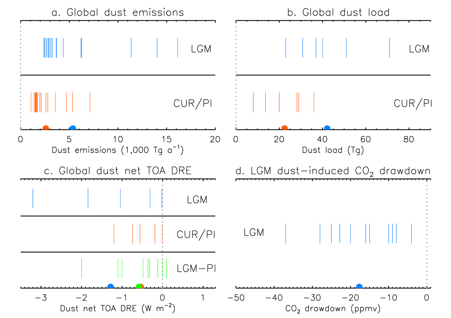
Figure 1: Synthesis of global metrics from LGM dust simulations, adapted from Albani et al. (2018). Vertical bars represent the results of individual experiments. The semi-circles on the x-axes mark the average of the respective model ensembles. The vertical gray dotted lines mark the zero value on the x-axis. CUR/PI indicates either current or pre-industrial simulations. TOA DRE stands for Top Of Atmosphere Direct Radiative Effect.

The paleoclimate dust community has strongly focused on the LGM period, owing to the large dust flux increase marked particularly in mid- and high-latitude paleoarchives. However, only a few modeling groups have tried to simulate the LGM dust cycle, with a varying level of validation against modern and paleodata. Estimates of dust emissions, load, direct radiative effects, and impacts on the carbon cycle through iron fertilization are summarized in Figure 1. The large spread in results can mainly be attributed to differences in the representation of dust emission and deposition mechanisms, differences in boundary conditions (including vegetation), inclusion of glaciogenic (formed by glacier abrasion) dust sources, different aerosol size ranges and optical properties, and assumptions about dust-borne iron solubility and bioavailability.

Overall, the central estimates from these simulations suggest that global LGM dust probably doubled in load compared to the late Holocene. This likely contributed about 25% (–20 ppmv) to the CO₂ drawdown through iron fertilization of the oceans and had a direct radiative forcing of –0.6 W/m², slightly lower than the main other forcing mechanisms (greenhouse gases: –2.8 W/m², ice sheets and sea level changes: –3.0 W/m²; Albani et al. 2018). However, direct radiative forcing estimates of global dust average both positive and negative values; locally and regionally, the magnitudes can be much stronger (Albani and Mahowald 2019).

The mid-Holocene (MH) had received far less attention until recently, when it was found that marine sediment records indicated that North African dust emissions were two to five times lower during the "green Sahara" phase than during the late Holocene. These findings motivated the first efforts to simulate and reconstruct the MH global dust cycle (Albani et al. 2015). New idealized and realistic experiments quickly followed, highlighting the role of dust on the ITCZ and monsoon dynamics (e.g. Albani and Mahowald 2019; Braconnot et al. 2021; Hopcroft et al. 2019).

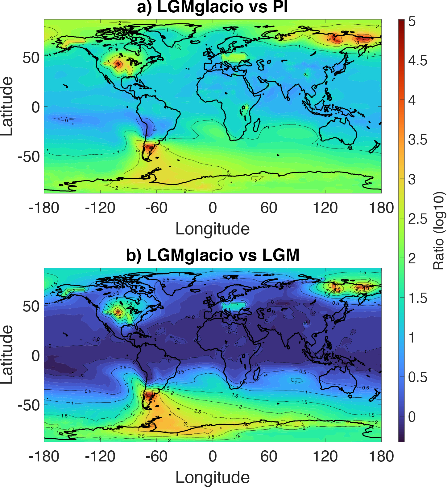
Figure 2: Simulated surface dust deposition ratios (Ohgaito et al. 2018). (A) Ratio of the LGM simulation including glaciogenic sources to the PI simulation; (B) ratio of the LGM simulations with and without glaciogenic sources (note the logarithmic ratio scale).

Although the aforementioned simulations were performed using PMIP climate models (or adaptations thereof), it was only recently that CMIP/PMIP protocols started to include dust forcings beyond the use of prescribed pre-industrial (PI) or present day (PD) fields. The importance of replacing the PI and PD fields with period-accurate fields (including additional glaciogenic sources in LGM simulations) is evidenced in Figure 2, with LGM surface dust depositions generally several orders of magnitude larger than during the PI period. Although the inclusion of glaciogenic sources in LGM simulations may not appear crucial for global radiative forcing, they are very important for local and indirect effects (Lambert et al. 2021).

The new CMIP6/PMIP4 protocol allows for dust to vary across climates, either as a prognostically emitted species, or prescribed based on previous paleoclimate simulations or reconstructions (Kageyama et al. 2017; 2018; Otto-Bliesner et al. 2017). As the first PMIP4 papers focused on dust begin to emerge (Braconnot et al. 2021), these efforts are leading to a new exciting phase. We hope that soon many more groups will start to contribute to the effort of understanding the role of dust in the climate system, both as a tracer of past changes of land-surface and atmospheric conditions, as well as an active agent affecting local, regional, and global climate in various ways.

Future Directions

Recent studies have investigated more complex and detailed dust-climate interactions. These include the dust-vegetation-monsoon nexus (Hopcroft et al. 2019), the effects of dust on snow albedo (Albani and Mahowald 2019; Mahowald et al. 2006; Ohgaito et al. 2018), and the regional features of dust on biogeochemistry, radiative effects and forcing, as well as the dynamical response of the climate system to these forcings (Albani and Mahowald 2019; Braconnot et al. 2021; Lambert et al. 2021).

The newest generation of climate models feature developments of great interest for paleoclimatic dust simulations. These include the incorporation of more realistic particle sizes and optical properties (Albani and Mahowald 2019; Hopcroft et al. 2019) and indirect effects on clouds (Ohgaito et al. 2018), as well as coupling of dust to ocean biogeochemistry, iron processing during atmospheric transport, and explicit representation of particle mineralogy (Hamilton et al. 2019). In its latest iteration, PMIP has been expanding from the mainstay MH and LGM periods to include further equilibrium simulations and transient simulations. Transient simulations are of particular interest to the dust community to investigate the variability and timing of occasional abrupt variations recorded in dust records. These were shown to potentially affect the global carbon cycle on short timescales (Lambert et al. 2021), and additional short-term feedbacks are likely.

To meet future challenges as a community, it is important to highlight the need for interaction and cooperation between the empirical and modeling communities. We stress the need for feedback between the two for project planning. Data syntheses are an important and necessary bridge between empirical measurements and simulations. Ongoing work is expanding the existing Holocene dust synthesis (Albani et al. 2015) to provide a comprehensive dust database of timeseries of dust-mass accumulation rates, with information about the particle-size distribution, over the last glacial-interglacial cycle; it is hoped that this will address some of the needs of the paleoclimate modeling community.

Recently, a new PMIP focus group on dust was launched, with the aims to: (1) coordinate a dust synthesis from PMIP4 experiments and (2) promote the definition of the experimental design for CMIP7/PMIP5 dust experiments. The group may also provide data as a benchmarking tool and boundary conditions for future equilibrium and transient simulations, should this be aligned with the scopes of the next phase. Interested parties are encouraged to contact the authors to participate in this effort.

affiliations

1Department of Physical Geography, Pontificia Universidad Católica de Chile, Santiago, Chile

2Millennium Nucleus Paleoclimate, University of Chile, Santiago, Chile

3Center for Climate and Resilience Research, University of Chile, Santiago, Chile

4Department of Environmental and Earth Sciences, Università degli Studi di Milano-Bicocca, Milan, Italy

contact

Fabrice Lambert: lambertuc.cl

references

Albani S, Mahowald NM (2019) J Clim 32: 7897-7913

Albani S et al. (2015) Clim Past 11: 869-903

Albani S et al. (2018) Curr Clim Change Rep 4: 99-114

Braconnot P et al. (2021) Clim Past 17: 1091-1117

Hain MP et al. (2014) In: Holland H, Turekian K (Eds) Treatise on Geochemistry. Elsevier, 485-517

Hamilton DS et al. (2019) Geosci Model Dev 12: 3835-3862

Hopcroft PO, Valdes PJ (2019) Geophys Res Lett 46: 1612-1621

Joussaume S (1993) J Geophys Res Atmos 98: 2767-2805

Kageyama M et al. (2017) Geosci Model Dev 10: 4035-4055

Kageyama M et al. (2018) Geosci Model Dev 11: 1033-1057

Lambert F et al. (2021) Earth Planet Sci Lett 554: 116675

Maher BA et al. (2010) Earth Sci Rev 99: 61-97

Mahowald NM et al. (2006) J Geophys Res 111: D10202

Ohgaito R et al. (2018) Clim Past 14: 1565-1581

Otto-Bliesner BL et al. (2017) Geosci Model Dev 10: 3979-4003

Prospero JM et al. (2002) Rev Geophys 40: 1002

Sam Sherriff-Tadano¹ and Marlene Klockmann²

Simulations of the Last Glacial Maximum (LGM) within PMIP significantly improved our understanding of the mechanisms that control the Atlantic Meridional Overturning Circulation (AMOC) in a glacial climate. Nonetheless, reproducing the reconstructed shallowing of the LGM AMOC remains a challenge for many models.

AMOC at the LGM

The Last Glacial Maximum (LGM; ca. 21,000 years ago) was a period within the last glacial cycle with very low greenhouse gas concentrations and maximum ice volume. The global climate was much colder than the modern climate, and the state of the Atlantic Meridional Overturning Circulation (AMOC) was very different as a consequence of the glacial climate forcings. In the modern climate, North Atlantic Deep Water (NADW), which forms in the Nordic and Labrador Seas, fills the deep North Atlantic basin. In contrast, proxy data such as carbon and neodymium isotopes, suggest that during the LGM, a large fraction of NADW in the deep Atlantic basin was replaced by Antarctic Bottom Water (AABW), which is formed in the Southern Ocean. As a result, the glacial AMOC was shallower than the modern AMOC (Lynch-Stieglitz 2017). The strength of the LGM AMOC is harder to reconstruct; proxies of AMOC strength support a glacial AMOC state ranging from weaker than or similar to today (e.g. Lynch-Stieglitz 2017). Nonetheless, the LGM provides a good opportunity to understand the AMOC response to climate changes as well as to evaluate the capability of comprehensive atmosphere-ocean coupled general circulation models (AOGCM) to reproduce AMOC states which are very different from today.

LGM AMOC from PMIP1 to PMIP4

Throughout the four PMIP phases, simulating the LGM AMOC has remained a challenge. While the respective AOGCMs tend to agree on large-scale changes in surface cooling patterns, the simulated AMOC changes differ strongly between models and PMIP phases, and most models cannot simulate the reconstructed shallower LGM AMOC. The first official LGM AMOC model intercomparison was conducted as part of PMIP2 (Weber et al. 2007); this intercomparison included three additional simulations from AOGCMs that adopted the PMIP1 protocol. These simulations are referred to as PMIP1.5 simulations. Here, we include a fourth PMIP1.5-type simulation (Kim 2004) that was not part of the original intercomparison.

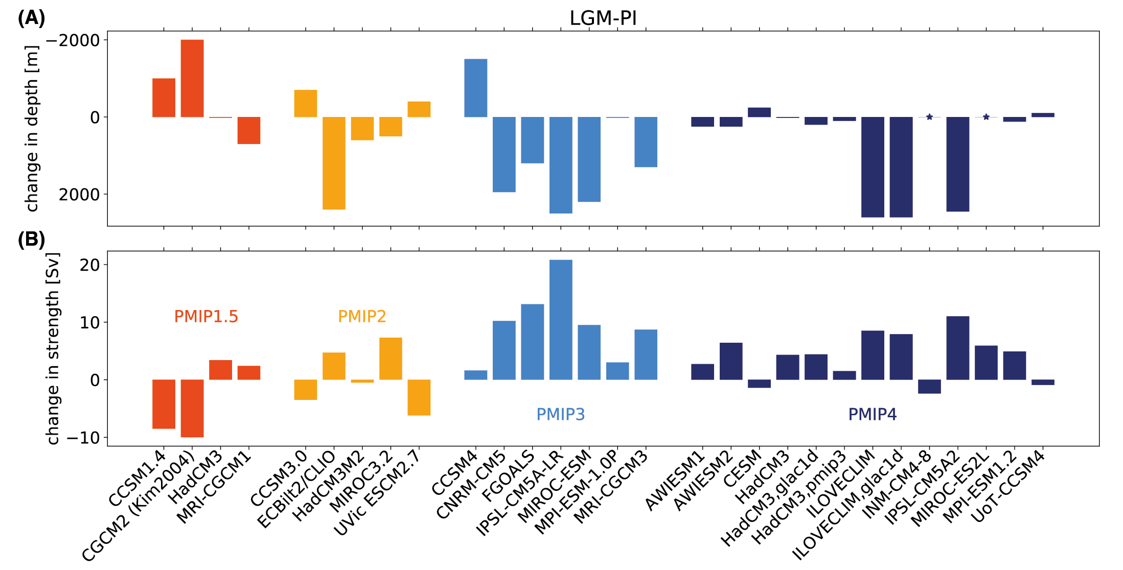
In Figure 1, the results of various PMIP phases are shown. Out of nine PMIP1.5/PMIP2 models, four simulated a shallower and weaker LGM AMOC, three a stronger and deeper LGM AMOC, one simulated a stronger LGM AMOC with no changes in depth, and one a deeper and slightly weaker LGM AMOC. In PMIP3, the inter-model spread was much smaller, but fewer models agreed with reconstructions. Only one model simulated a shallower LGM AMOC, one simulated no change in depth, and all other models simulated a much deeper LGM AMOC. All models simulated a stronger LGM AMOC. In PMIP4, most models simulated a stronger LGM AMOC, while all but two models simulated very minor changes in the depth (Kageyama et al. 2021).

Figure 1: (A) AMOC depth and (B) strength at the LGM compared to pre-industrial (PI) in the PMIP generations 1.5–4. The values for PMIP1.5 and PMIP2 are taken from Weber et al (2007) and Kim (2004); values for PMIP3 and PMIP4 are taken from Kageyama et al (2021). AMOC strength is defined as the maximum transport in Sv at 30°N. AMOC depth is defined as the depth of the interface between the NADW and AABW cell at 30°N for CGCM2, PMIP3, and PMIP4, and at the Southern end of the Atlantic basin for PMIP1.5 and PMIP2. Negative values in AMOC depth and strength correspond to shoaling and weakening of LGM AMOC compared to PI. Asterisks indicate that the NADW cell covers the entire water column in both PI and LGM simulations.

What have we learned from PMIP?

The PMIP ensembles have provided many plausible hypotheses regarding the mechanisms that control the LGM AMOC. While there are still open questions, it is possible to assemble some pieces of the puzzle to form a consistent picture. The PMIP1.5/PMIP2 simulations suggested that the meridional density contrast between NADW and AABW source regions plays a key role in controlling the AMOC state (Weber et al. 2007): the glacial AABW needs to become much denser than the NADW in order to generate strong enough stratification in the deep ocean, thereby inducing a shallower AMOC. Starting from there, key processes that modify the meridional density gradient under LGM conditions can be identified.

In the Southern Hemisphere, buoyancy loss through sea-ice export and brine release in the Southern Ocean associated with low CO₂ concentrations are key for the formation of dense AABW (Klockmann et al. 2016). Models with a shallower LGM AMOC tend to have a very strong buoyancy loss over the Southern Ocean (Otto-Bliesner et al. 2007). An additional factor could be the duration of the spin-up: a sufficient integration time is required to account for the slow penetration and densification of the deep Atlantic by AABW (Marzocchi and Jansen 2017).

In the Northern Hemisphere, key processes are changes in the North Atlantic freshwater budget, sea-ice cover, and surface winds. Stronger LGM surface winds over the North Atlantic caused by the Laurentide ice sheet increase the density and formation of NADW and induce a strong and deep LGM AMOC (Muglia and Schmittner 2015; Sherriff-Tadano et al. 2018). Extensive sea-ice cover or increased freshwater input in the NADW formation sites reduces the buoyancy loss and leads to less dense NADW and a weaker and shallower AMOC (Oka et al. 2012; Weber et al. 2007). Depending on the model specifics, these mechanisms might compensate differently and lead to very different LGM states (Klockmann et al. 2018).

Few PMIP4 models simulate a substantial deepening of the LGM AMOC (Fig. 1). This improvement with respect to PMIP3 may imply that the models are making some progress in capturing the important processes and getting the balance right. Future analyses of the PMIP4 simulations will show whether this confidence is justified.

Discussion

The current ensemble of simulations across all PMIP phases contains 29 simulations from 26 different models. Only seven of these simulations capture the shallower LGM AMOC, and five were performed with models from the CCSM family (Fig.1). It is, therefore, reasonable to say that it remains a challenge for most AOGCMs to reproduce an LGM AMOC in agreement with reconstructions. Why is it so difficult?

There are several factors that affect the LGM AMOC, either because they affect the key mechanisms described above or through additional mechanisms. These factors are, for example, uncertainties in the ice-sheet reconstructions, the magnitude and representation of glacial tidal mixing (Peltier and Vettoretti 2014), or assumptions of the AMOC being in a quasi-equilibrium state with 21ka climate forcing (Zhang et al. 2013). The PMIP4 protocol explicitly addressed the uncertainties in the ice-sheet reconstructions by offering a choice between three different reconstructions: ICE6G, GLAC1D, and the previous PMIP3 ice sheets (Kageyama et al. 2017 and references therein). Most PMIP4 simulations were run with the ICE6G ice sheets; only two models were used for multiple simulations with different ice sheets. In these two models, the different ice-sheet reconstructions make only a small difference for the simulated LGM AMOC, but this need not be the case for other models or other ice-sheet reconstructions.

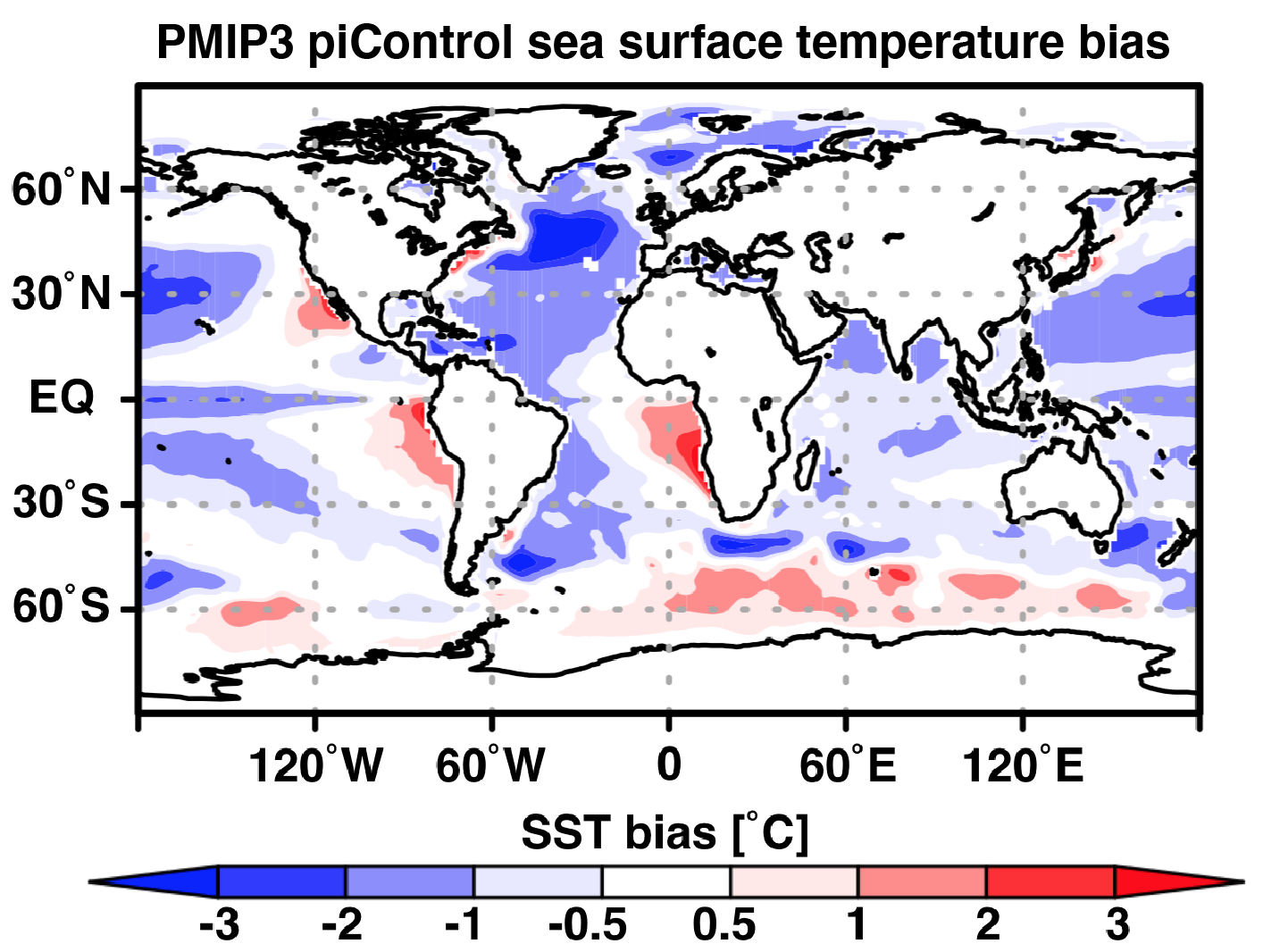
Figure 2: PMIP3 model mean annual sea-surface temperature bias in pre-industrial climate simulations compared with World Ocean Atlas 2013 (nodc.noaa.gov/OC5/woa13/woa13data.html).

Additional problems could arise from biases in the pre-industrial control simulations. Figure 2 shows sea-surface temperature (SST) biases in pre-industrial climate simulations from PMIP3 models. Large SST biases are evident over the Southern Ocean and northern North Atlantic, where AABW and NADW are formed, respectively. A recent study with an AOGCM showed, in fact, that an improvement in modern SST biases over the Southern Ocean could help to reproduce the shallower LGM AMOC by enhancing the formation of AABW (Sherriff-Tadano et al. submitted). NADW formation areas experience large changes in surface winds at the LGM; hence, biases in this region require additional attention as well.

In the future, sensitivity experiments such as parameter ensembles, or partially coupled experiments, may provide useful information regarding the role of uncertain climate parameters and model biases in LGM simulations. Increased direct modeling of carbon isotopes and relevant tracers will be key for model–data comparisons, and to better understand and constrain the LGM AMOC, including its strength.

affiliations

¹School of Earth and Environment, University of Leeds, UK

²Institute of Coastal Systems – Analysis and Modelling, Helmholtz-Zentrum Hereon, Geesthacht, Germany

contact

Sam Sherriff-Tadano: S.Sherriff-Tadanoleeds.ac.uk

Marlene Klockmann: marlene.klockmannhereon.de

references

Kageyama M et al. (2017) Geosci Model Dev 10: 4035-4055

Kageyama M et al. (2021) Clim Past 17: 1065-1089

Kim SJ (2004) Clim Dyn 22: 639-651

Klockmann M et al. (2016) Clim Past 12: 1829-1846

Klockmann M et al. (2018) J Clim 31: 7969–7984

Lynch-Stieglitz J (2017) Ann Rev Mar Sci 9: 83-104

Marzocchi A, Jansen MF (2017) Geophys Res Lett 44: 6286-6295

Muglia J, Schmittner A (2015) Geophys Res Lett 42: 9862-9869

Oka A et al. (2012) Geophys Res Lett 39: L09709

Otto-Bliesner B et al. (2007) Geophys Res Lett 34: 6

Peltier R, Vettoretti G (2014) Geophys Res Lett 41: 7306-7313

Sherriff-Tadano S et al. (2018) Clim Dyn 50: 2881-2903

Weber S et al. (2007) Clim Past 3: 51-64

Zhang X et al. (2013) Clim Past 9: 2319-2333

Lukas Jonkers¹, K. Rehfeld^2,3, M. Kageyama⁴ and M. Kucera¹

The Last Glacial Maximum (LGM) offers paleoscientists the possibility to assess climate model skill under boundary conditions fundamentally different from today. We briefly review the history and challenges of LGM data–model comparison and outline potential new future directions.

The Last Glacial Maximum

The Last Glacial Maximum (LGM; 23,000–19,000 years ago) is the most recent time in Earth's history with a fundamentally different climate from today. Thus, from a climate modeling perspective, the LGM is an ideal test case because of its radically different and quantitatively well-constrained boundary conditions.

Reconstructions provide quantitative constraints on LGM climate, but they are often archived in isolation. Paleoclimate syntheses bring individual reconstructions together and offer a large-scale, even global, perspective on paleoclimate that is impossible to obtain from single observations. The first synthesis of the LGM surface temperature field, carried out within the Climate: Long range Investigation, Mapping, and Prediction (CLIMAP) project in the 1970s, served as boundary conditions for atmosphere-only models (CLIMAP Project Members 1976), which required full-field seasonal reconstructions. Later, with the advent of coupled ocean-atmosphere models, the information from paleoclimate archives could be used to benchmark simulations.

Since CLIMAP, the data coverage has increased tremendously and new (geochemical) proxies for seawater temperature have been developed and successfully applied. Thanks to synthesis efforts, the LGM is now arguably the time period with the most extensively constrained sea-surface temperature field prior to the instrumental period (MARGO project members 2009; Tierney et al. 2020).

Climate models largely capture the reconstructed global average LGM cooling of the oceans (Kageyama et al. 2021; Otto-Bliesner et al. 2009), thus allowing us to constrain climate sensitivity (Sherwood et al. 2020). However, the average LGM cooling emerges from a signal of marked variability (MARGO project members 2009; Rehfeld et al. 2018), a reflection of climate dynamics that cannot be resolved from the global mean. The reconstructions indicate pronounced regional patterns of the oceanic temperature change, with, amongst others, pronounced gradients in the cooling in the North Atlantic (MARGO project members 2009). It is in the spatial patterns of LGM temperature change where there are the largest differences among the individual proxies and models, as well as between the proxies and the models (Kageyama et al. 2021).

The causes—and hence implications—for these differences (and model–data mismatch in general) arise from both the reconstructions and the models. It is important to resolve the underlying reasons for the differences in order to increase the relevance of paleodata model comparison for future predictions.

Main challenges

A crucial first step to assess (any) mismatch between paleoclimate reconstructions and simulations is to quantify the uncertainty and bias of both. Without this, the reason for differences (or the meaning of agreement) will remain difficult to elucidate.

Paleoclimate records preserve an imprint of past climate that is affected by uncertainty in the chronology of the archives and in the attribution of the signal together with additional noise that may be unrelated to climate. Previous work suggests that—at least for the LGM—dating uncertainties and internal variability are not the largest source of error for the reconstructions (Kucera et al. 2005). This is likely because sediment records are averaged enough across the four millennia that span the LGM, and the dating aided by the radiocarbon technique is sufficiently reliable to identify the target time slice. Instead, the attribution of the reconstructed temperatures to specific water depths or seasons, as well as the influence of factors other than temperature on the proxy signals, remain problematic and likely explain part of the difference among proxies (Fig. 1c).

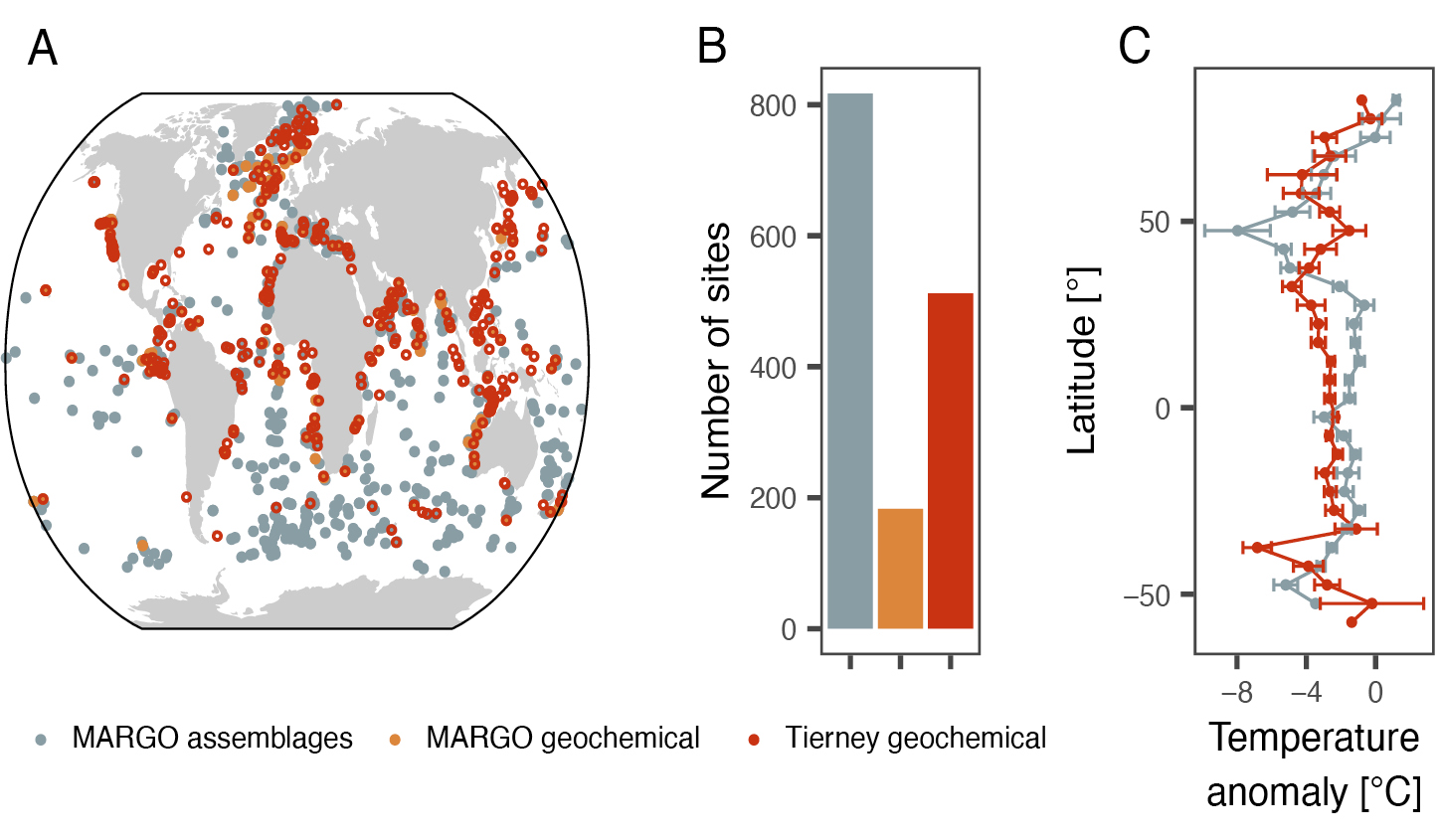
Figure 1: (A,B) Sites with LGM sea surface temperature reconstruction in the MARGO project members (2009) and Tierney et al. (2020) compilations and (C) binned latitudinal mean annual temperature anomaly with respect to the present day derived from assemblages-based and geochemical proxies. Errorbars represent standard errors of the mean.

Climate model simulations, on the other hand, are physically plausible realizations of climate dynamics that are simplifications of reality, a fundamental aspect that should not be forgotten during data–model comparison. Models are generally calibrated to instrumental data so that LGM simulations are independent tests of their ability to represent a climate different from the present. Model design choices lead to differences among the simulations of LGM temperature that are on a par with differences among proxies (Fig. 2). Among these design choices, the coarse spatial resolution of climate models leads to difficulties in accurately resolving small-scale features, such as eastern boundary currents or upwelling systems: areas where the data–model mismatch tends to be large (Fig. 2). Moreover, modelers have to make choices in terms of boundary conditions (in particular ice sheets) and in the set-up of the model used (e.g. including dynamic vegetation, interactive ice sheets). And finally, most simulations of LGM climate are performed as equilibrium experiments (without history/memory), whereas in reality the LGM was the culmination of a highly dynamic glacial period.

Ways forward

Proxy attribution can be addressed directly through increased understanding of the proxy sensor. Most seawater temperature proxies are based on biological sensors, and better understanding of their ecology is likely to help constrain the origin of the proxy signal (Jonkers and Kucera 2017). Alternatively, uncertainty in the attribution may also be accounted for in the calibration (e.g. Tierney and Tingley 2018). However, neither approach explicitly considers the dependence of the proxy sensor itself on climate. Forward modeling of the proxy signal is a promising way to address this issue, but sensor models for seawater temperature proxies are still in their infancy (Kretschmer et al. 2018).

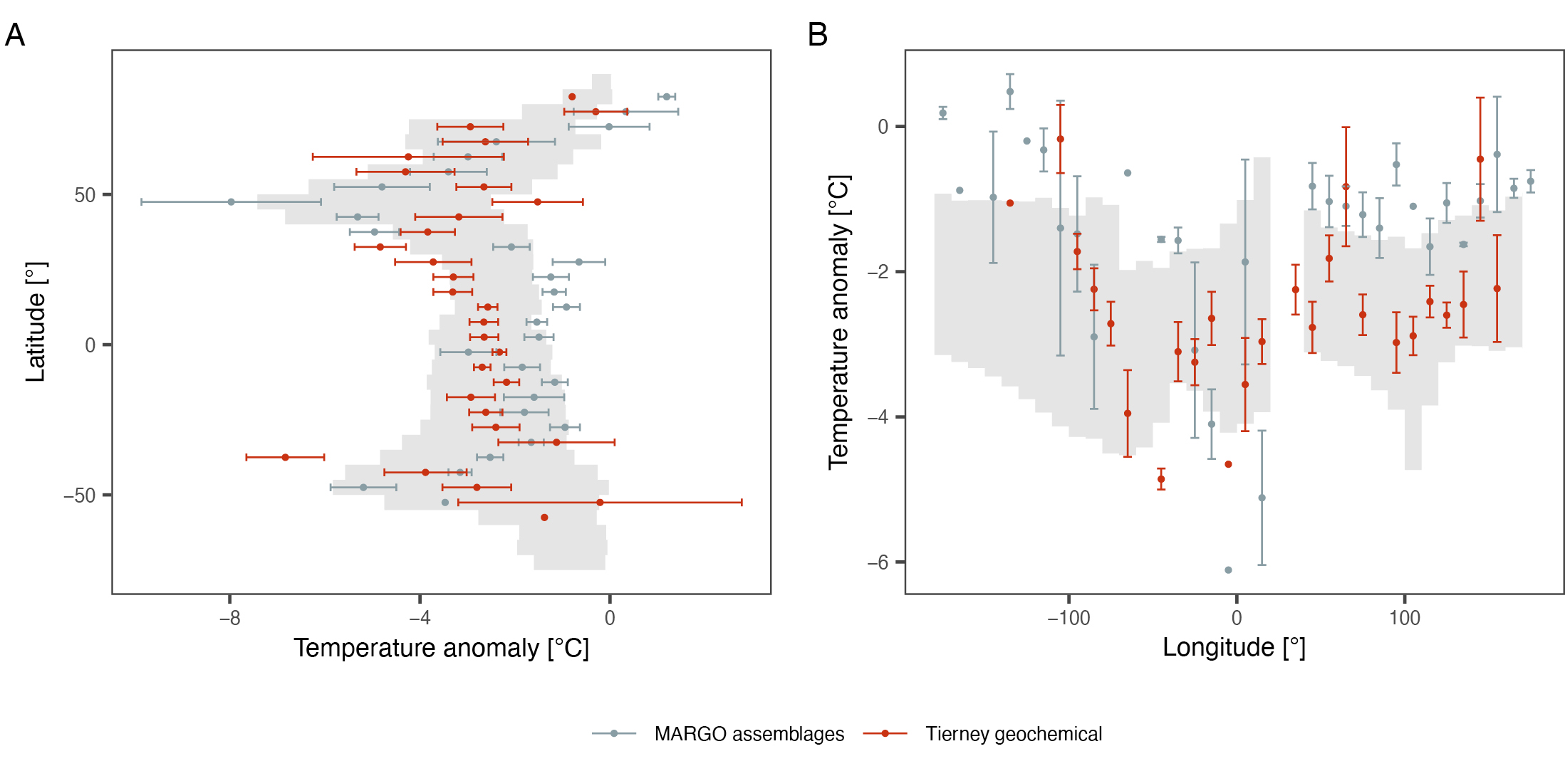
Figure 2: (A) Zonal and (B) tropical meridional (15°N–15°S) mean annual LGM sea surface temperature anomalies in reconstructions (colors) compared to PMIP4 inter-model spread (gray background). Reconstructions and simulations are binned at the same resolution; errorbars represent standard errors of the mean.

Apart from the proxy attribution uncertainties, reconstructions are spatially distributed in an uneven way. For both historical and geological reasons most of the reconstructions stem from the North Atlantic Ocean and from continental margins (Fig. 1) and despite almost half a century of focus on reconstructing the LGM temperature field, progress in filling the gaps has been slow. This is in part due to the depositional regime that characterizes large parts of the open ocean. Sedimentation rates and/or preservation in these areas are often insufficient to resolve the LGM. Therefore, it would seem that rather than aiming for a reconstruction of global mean temperature, a more fruitful approach would be to focus on areas where the reconstructions can better constrain the simulations, for instance in areas where models show the largest spread or bias.

At the same time, uncertainty, including structural uncertainty in model simulations has to be considered more explicitly. It is now more and more common to run large ensembles of model simulations, thereby sampling parametric uncertainties and/or uncertainties in scenarios, or in initial or boundary conditions. Such an approach, together with the multi-model approach that PMIP has fostered, helps to better describe the uncertainty of the model simulations, and better quantify model–data (dis)agreement. Taking uncertainty in the models and in the paleodata into account, simulations and reconstructions can be integrated through data assimilation (Kurahashi-Nakamura et al. 2017; Tierney et al. 2020). Offline approaches to obtain full field reconstructions are valuable but difficult to validate. Furthermore, such methods require some overlap between reconstructions and simulations to obtain reconstructions that are not only physically plausible but also realistic. Online data assimilation is possibly the most direct way of using the strengths of the models and the data to learn about the climate system.

Outlook

Avenues to increase the value of paleoclimate data to inform climate models would be to better exploit the multidimensionality of the paleorecord. Archives of marine climate often hold more information than just temperature. Because many archives co-register different climate-sensitive parameters, (age) uncertainty can be reduced to some extent. Thus, approaches carrying out comparison, or data assimilation, in multiple dimensions (Kurahashi-Nakamura et al. 2017) are likely to provide more constraints on the reason for model–data discrepancies.

Although the LGM time slice has proved a useful and effective way to compare models and data, the paleoclimate record is in fact four-dimensional, as it traces changes through time and space. Climate models can now increasingly simulate transient change over long periods of time. The future of climate model–data integration therefore likely belongs to timeseries comparisons (Ivanovic et al. 2016). Timeseries can be used to assess the temporal aspect of climate variability and the large-scale evolution of climate. With the increasing availability of multi-proxy/parameter data synthesis (Jonkers et al. 2020), even the prospect of four-dimensional data–model comparison is coming closer to reality.

affiliations

¹MARUM Center for Marine Environmental Sciences, University of Bremen, Germany

²Geo- und Umweltforschungszentrum, Tübingen University

³Institute of Environmental Physics, Heidelberg University, Germany

⁴Laboratoire des Sciences du Climat et de l'Environnement, Institut Pierre-Simon Laplace, UMR CEA-CNRS-UVSQ, Université Paris-Saclay, Gif-sur-Yvette, France

contact

Lukas Jonkers: ljonkersmarum.de

references

CLIMAP Project Members (1976) Science 191: 1131-1137

Ivanovic RF et al. (2016) Geosci Model Dev 9: 2563-2587

Jonkers L, Kucera M (2017) Clim Past 13: 573-586

Jonkers L et al. (2020) Earth Syst Sci Data 12: 1053-1081

Kageyama M et al. (2021) Clim Past 17: 1065-1089

Kretschmer K et al. (2018) Biogeosciences 15: 4405-4429

Kucera M et al. (2005) Quat Sci Rev 24: 951-998

Kurahashi-Nakamura T et al. (2017) Paleoceanography 32: 326-350

MARGO project members (2009) Nat Geosci 2: 127-132

Otto-Bliesner BL et al. (2009) Clim Dyn 32: 799-815

Rehfeld K et al. (2018) Nature 554: 356-359

Sherwood SC et al. (2020) Rev Geophys 58: e2019RG000678

Tierney JE, Tingley MP (2018) Paleoceanogr Paleoclimatol 33: 281-301

Tierney JE et al. (2020) Nature 584: 569-573

Masa Kageyama¹, A. Abe-Ouchi², T. Obase², G. Ramstein¹ and P.J. Valdes³

The Last Glacial Maximum is an example of an extreme climate, and has thus been a target for climate models for many years. This period is important for evaluating the models' ability to simulate changes in polar amplification, land–sea temperature contrast, and climate sensitivity.

The Last Glacial Maximum (LGM, ∼21,000 years ago), a period during which the global ice volume was at a maximum and global eustatic sea level at a minimum, inspired some of the first simulations of past atmospheric circulation and climates (Gates 1976; Manabe and Broccoli 1985a; Manabe and Broccoli 1985b; Kutzbach and Wright 1985). Because of the extreme conditions during this period, the LGM was documented quite early, notably through the CLIMAP project (e.g. CLIMAP Project Members 1981). This early work gave rise to many questions: how cold, how dry, how dusty was it, and why? How was the Northern Hemisphere ice sheet sustained? How did the massive ice sheet impact the atmospheric and oceanic circulation? What were the impacts of these ice sheets on climate, compared to the impact of other changes in forcings and boundary conditions, such as the decrease in greenhouse gas concentrations? What climate feedbacks were induced by vegetation, the cryosphere, dust, and permafrost? Are the features from paleodata reconstructions also found in the results of the models that are routinely used to compute present and future climate changes? Climate reconstructions for the LGM were also hotly debated, sometimes in relation to one another, such as for tropical cooling over sea and over land (e.g. Rind and Peteet 1985).

In the beginning

PMIP was launched as a result of a NATO Advanced Research Workshop in Saclay, France, in 1991 (Joussaume and Taylor, this issue). At that time, several LGM simulations had already been carried out, and the different modeling groups involved in running these experiments had therefore already gathered some experience. However, these simulations were not strictly comparable since they did not use the same forcings or boundary conditions. For example, the CO₂ forcing, which became a central point of LGM climate analyses due to its connection with climate sensitivity, was actually not taken into account in climate simulations until the work of Manabe and Broccoli (1985b), who cited the CO₂ retrieved from Greenland and Antarctic ice cores published by Neftel et al. (1982). At the Saclay meeting, it was clear that many groups of modelers and data scientists were motivated to build a common project to better understand the climate during the mid-Holocene and the Last Glacial Maximum, based on numerical simulations and on syntheses of paleoclimatic reconstructions.

Developing the approach

It took time, intensive debates, and several PMIP meetings to agree on a common approach, forcings and boundary conditions; develop a strategy for paleodata compilations; and establish a methodology for model–data comparison. Therefore, the real launch of the PMIP1 LGM simulations was in 1994. Despite having chosen to adopt an approach that would be as simple as possible, it took no fewer than four newsletters to describe the corresponding experimental protocol (pmip1.lsce.ipsl.fr/ > Newletters). To engage as many groups as possible in this new adventure, the decision was made to allow for two types of simulations to be run for the LGM: one using atmosphere-only general circulation models (AGCMs) and therefore prescribing surface conditions (sea surface temperatures and sea ice from the CLIMAP (1981) reconstructions), the other using AGCMs coupled to slab ocean models, which computed the ocean conditions under the (strong) assumption that the ocean heat transport was similar to the pre-industrial one.

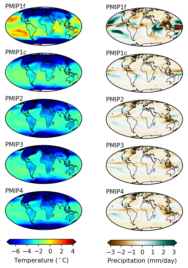
Figure 1: LGM – PI multi-model average anomalies simulated by climate models of the different PMIP phases for Mean Annual Temperature (left) and precipitation (right). PMIP1f: PMIP1-prescribed SST AGCM simulations; PMIP1c: simulations run with AGCMs coupled to slab ocean models. All other PMIP phases used coupled atmosphere-ocean GCMs.

The recommended ice-sheet reconstruction (ICE-4G; Peltier 1994) was the same for both types of experiments. Encouraging groups to run prescribed and computed SST experiments proved to be a wise decision, as this resulted in a total of eight simulations of each type being made available with contrasting results (Fig. 1). The largest difference between the groups of PMIP simulations is clearly between the prescribed SST simulations (labelled "PMIP1f") and the computed SST simulations (labelled "PMIP1c"). Both ensemble means show global cooling, amplified from the equator to the poles, with stronger cooling over the continents than over the oceans. These two large-scale characteristics (later termed "polar amplification" and "land–sea contrast") would be analyzed in all phases of PMIP, as these features are also seen in projections of future climate and should therefore be evaluated. Another topic of analysis was the atmospheric circulation in the vicinity of the large Northern Hemisphere ice sheets, following the striking "split-jet" response found in the pioneer, pre-PMIP simulations. This feature was not systematically found in the PMIP1 experiments, but the response of the atmospheric circulation and its interaction with the oceans remains a topic of active research.

What Figure 1 does not show is that the range of the PMIP1c results was much larger than that for PMIP1f, foreshadowing the need for coupled ocean-atmosphere models (cf. Braconnot et al. this issue). The advent of coupled ocean-atmosphere general circulation models resulted in the launch of the second phase of PMIP in 2002 (Harrison et al. 2002) with an updated ice-sheet boundary condition: ICE-5G (Peltier 2004; Fig. 2). Running these experiments was technically challenging, and it remains so because it forces the climate models out of their "comfort zone" (i.e. the conditions for which the models were initially developed). It requires a long equilibration time, which is very computationally expensive for the latest generation of models. Despite these challenges, the use of these coupled models proved to be very worthwhile, as they allowed for the use of marine data for evaluation, rather than for prescribing boundary conditions. This represented a huge release of the constraints on ocean reconstructions, which did not need to cover all the world's oceans for winter and summer. New ways to compare models and marine data became available, taking into account the indicators' specificities, some of which are still being investigated today. These should help us understand why reconstructions from different indicators sometimes differ significantly (Jonkers et al. this issue).

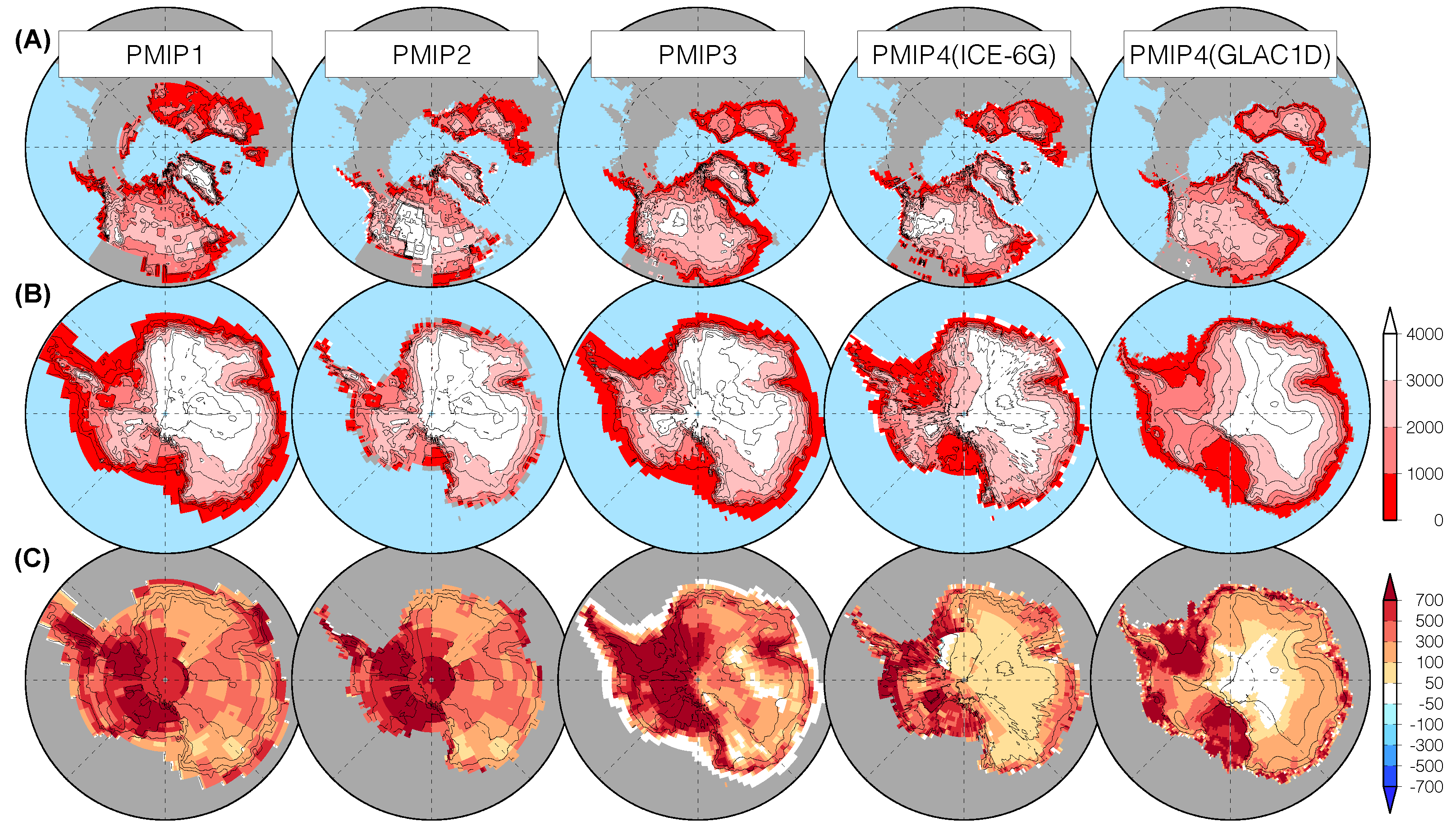
Figure 2: Evolution of the ice sheets used as boundary condition in the different PMIP phases. From the left to right: PMIP1 (ICE-4G; Peltier 1994), PMIP2 (ICE-5G; Peltier 2004), PMIP3 (Abe-Ouchi et al. 2005), PMIP4 (ICE-6G_C; Argus et al. 2014; Peltier et al. 2015), and PMIP4 (GLAC-1D; Ivanovic et al. 2016). (A) The altitude of Northern Hemisphere ice sheets at the LGM; (B) the altitude of Antarctica ice sheet at the LGM; (C) the altitude difference (LGM minus present day).

Progress in PMIP3 and PMIP4

Simulations during the third and fourth phases of PMIP were also run with coupled models, sometimes even with interactive vegetation, dust (see Lambert et al. this issue), and/or a carbon cycle (see Boutttes et al. this issue). While PMIP2 often used lower resolution models compared to those used for future climate projections, the novelty from PMIP3 onwards was that exactly the same model versions were used for both exercises, hence allowing for rigorous comparisons of processes involved in past and future climate changes. Boundary conditions, in particular in terms of ice-sheet reconstructions, were updated for each phase (Fig. 2). Ice-sheet reconstructions for the LGM were a hotly debated topic, but during the first three phases of PMIP, a single reconstruction was chosen. For PMIP3, this reconstruction was derived from three different reconstructions (Abe-Ouchi et al. 2015; Fig 2). Choosing a single protocol was deemed important for all the simulations to be comparable. For PMIP4, however, evaluating the uncertainty in model results related to the chosen boundary conditions was deemed necessary because differences between the ice-sheet reconstructions remained quite large in terms of ice-sheet altitude (Ivanovic et al. 2016; Kageyama et al. 2017). The PMIP4 dataset should ultimately help us reach this goal (most simulations presently available use Peltier's ICE-6G_C reconstruction; Argus et al. 2014; Peltier et al. 2015).

Providing an exhaustive list of the analyses based on these simulations would require more space than is available here. Recurring topics across the four phases of PMIP encompass large-scale to global features, such as climate sensitivity; polar amplification and land–sea contrast; atmosphere and oceanic circulation, in particular the Atlantic Meridional Overturning Circulation; the comparison of model results with reconstructions for various regions; and impacts on the ecosystems. An intriguing feature is that from PMIP2 to PMIP4, even though both models and experimental protocol have evolved, the range of model results (cf. Braconnot et al. this issue regarding the multi-model results in terms of cooling over tropical land and oceans) is quite stable, and within the range reconstructed from marine and terrestrial data. This might sound satisfactory, but in fact is a call for the reduction in the uncertainty of the reconstructions, the reconciliation of reconstructions from different climate indicators, or a better understanding of the differences and a refinement of the methodology regarding model–data comparisons. This would allow us to draw many more conclusions about the LGM in terms of understanding the climate system's sensitivity to changing forcings, and in terms of impacts of climate changes on the environments.

affiliations

¹Laboratoire des Sciences du Climat et de l'Environnement, LSCE/IPSL, UMR CEA-CNRS-UVSQ, Université Paris-Saclay, Gif sur Yvette, France

²Atmosphere and Ocean Research Institute, The University of Tokyo, Japan

³School of Geographical Sciences, University of Bristol, UK

contact

Masa Kageyama: Masa.Kageyamalsce.ipsl.fr

references

Abe-Ouchi A et al. (2015) Geophys Model Dev 8: 3621-3637

Argus DF et al. (2014) Geophys J Int 198: 537-563

Peltier WR et al. (2015) J Geophys Res Solid Earth 120: 450-487

CLIMAP Project Members (1981) Seasonal reconstruction of the Earth's surface at the last glacial maximum. Geol Soc Am, Map and Chart Series, p. 1-18

Gates WL (1976) Science 191: 1138-1144

Harrison SP et al. (2002) Eos 83: 447-447

Ivanovic RF et al. (2016) Geosci Model Dev 9: 2563-2587

Kageyama M et al. (2017) Geosci Model Dev 10: 4035-4055

Kutzbach JE, Wright HE (1985) Quat Sci Rev 4: 147-187

Manabe S, Broccoli AJ (1985a) J Geophys Res Atmos 90: 2167-2190

Manabe S, Broccoli AJ (1985b) J Atmos Sci 42: 2643-2651

Neftel A et al. (1982) Nature 295: 220-223

Peltier WR (1994) Science 265: 195-201

Peltier WR (2004) Annu Rev Earth Planet Sci 32: 111-149

Rind D, Peteet D (1985) Quat Res 24: 1-22

Ruza F. Ivanovic¹, E. Capron² and L.J. Gregoire¹

Recent cold-to-warm climate transitions present one of the hardest tests of our knowledge of environmental processes. In coordinating transient experiments of these elusive events, the Deglaciations and Abrupt Changes (DeglAC) Working Group is finding new ways to understand climate change.

Our journey to the present

In December 2010, amidst mountains of tofu, late-night karaoke stardom, and restorative trips to the local onsen (hot springs), the PMIP3 meeting in Kyoto, Japan (pastglobalchanges.org/calendar/128657), was in full swing. Results were emerging from transient simulations of the last 21,000 years attempting to capture both the gradual deglaciation towards present day climes and the abrupt aberrations that punctuate the longer-term trend. However, most of these experiments had employed different boundary conditions, and the models were showing different sensitivities to the imposed forcings. It was proposed that to better understand the last deglaciation, we should pool resources and develop a multi-model intercomparison project (MIP) for transient simulations of the period. This was a new kind of challenge for PMIP, which previously had focused mainly on equilibrium-type simulations (the last millennium experiment is a notable exception) of up to a few thousand years in duration. Fast forward to the present: DeglAC has its first results from its last deglaciation simulations. Eleven models of varying complexity and resolution have completed 21–15 kyr BP, with five of those running to 1950 CE or into the future.

Defining a flexible protocol

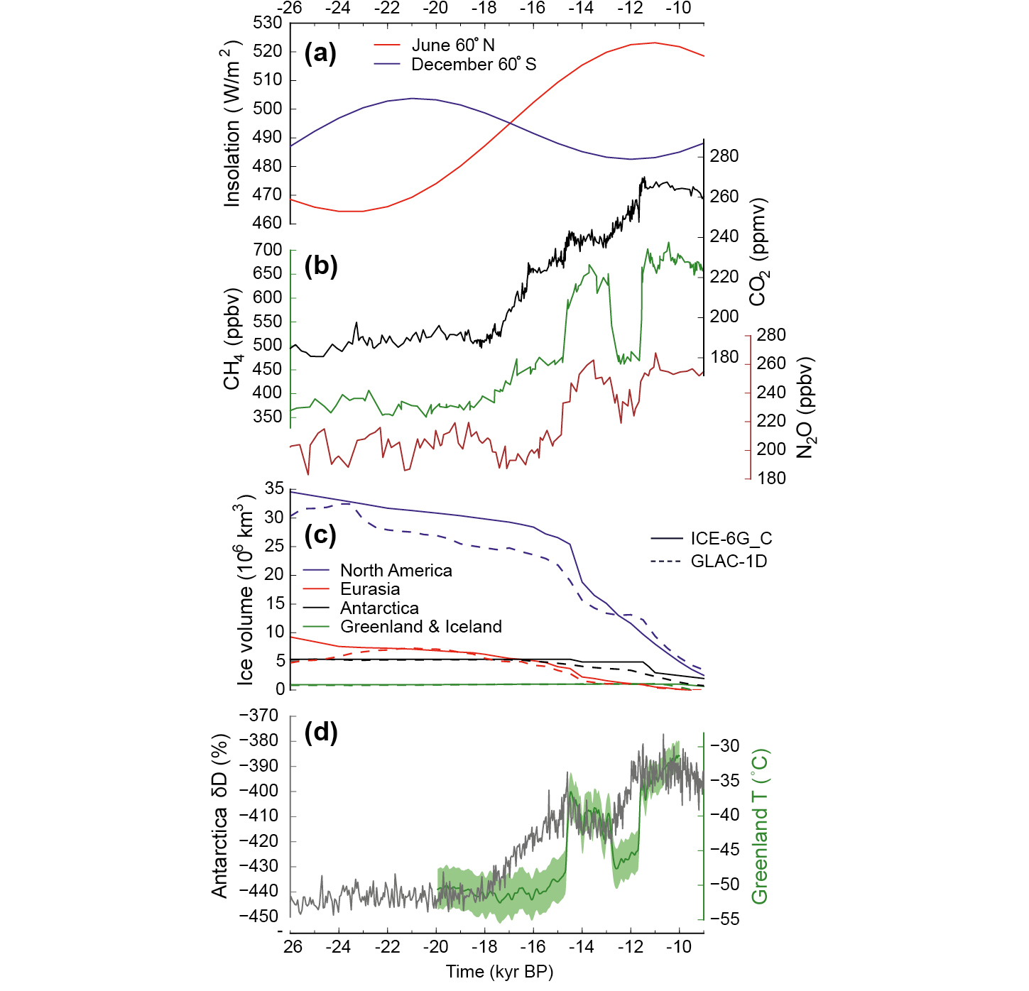
Real headway was made in 2014, when the PMIP3 meeting in Namur, Belgium (pastglobalchanges.org/calendar/128658), marked the inauguration of the DeglAC Working Group. That summer, the leaders of the Working Group made an open call for state-of-the-art, global ice-sheet reconstructions spanning 26–0 kyr BP, and two were provided: GLAC-1D and ICE-6G_C (VM5a). For orbital forcing, we adopted solutions consistent with previous PMIP endeavors, but the history of atmospheric trace gases posed some interesting questions. For instance, the incorporation of a new high-resolution record in a segment of the longer atmospheric CO₂ composite curve (Bereiter et al. 2015) raised fears of runaway terrestrial feedbacks in the models and artificial spikiness from sampling frequency. A hot debate continued over the appropriate temporal resolution to prescribe, and in the end, we left it up to individual modeling groups whether to prescribe the forcing at the published resolution, produce a spline through the discrete points, or interpolate between data, as needed. See Figure 1 for an overview of the experiment forcings and Ivanovic et al. (2016) for protocol details and references.

Figure 1: (A-C) Boundary conditions for the DeglAC MIP core experiment (version 1); (D) East Antarctic Plateau ice core δD (a proxy for local surface air temperature) and Greenland surface air temperature. After Ivanovic et al. (2016); see references therein.

The elephant in the room was what to do with ice-sheet melting. It is well known that the location, rate, and timing of freshwater forcing is critical for determining its impact on modeled ocean circulation and climate (and the impact can be large, e.g. Roche et al. 2011; Condron and Winsor 2012; Ivanovic et al. 2017). Yet, these parameters remain mostly uncertain, especially at the level of the spatial and temporal detail required by the models.

We explored a contentious proposal to set target ocean and climate conditions instead of an ice-sheet meltwater protocol. Many models have different sensitivities to freshwater (Kageyama et al. 2013), and it was strongly suspected that imposing freshwater fluxes consistent with ice-sheet reconstructions would confound efforts to produce observed millennial-scale climate events (Bethke et al. 2012). Thus, specifying the ocean and climate conditions to be reproduced by the participant models would encourage groups to employ whatever forcing was necessary to simulate the recorded events. However, the more traditional MIP philosophy is to use tightly prescribed boundary conditions to enable a direct inter-model comparison of sensitivity to those forcings, as well as evaluation of model performance and simulated processes against paleorecords. If the forcings are instead tuned to produce a target climate/ocean, then by definition of the experimental design, the models will have been conditioned to get at least some aspect of the climate "right", reducing the predictive value of the result. Although useful for examining the climate response to the target condition, and for driving offline models of other Earth system components (e.g. ice sheets, biosphere, etc.), we already know that this approach risks requiring unrealistic combinations of boundary conditions, which complicates the analyses and may undermine some of the simulated interactions and teleconnections. Ultimately, the complex multiplicity in the interpretation of paleorecords made it too controversial to set definitive target ocean and climate states in the protocol. Therefore, we recommended the prescription of freshwater forcing consistent with ice-sheet evolution, and allowed complete flexibility for groups to pursue any preferred scenario(s).

Such flexibility in uncertain boundary conditions is not the common way to design a paleo MIP, but this less traditional method is eminently useful. First and foremost, not being too rigid on model boundary conditions allows for the use of the model ensemble for informally examining uncertainties in deglacial forcings, mechanisms, and feedbacks. There are also technical advantages: the last deglaciation is a very difficult simulation to set up, and can take anything from a month to several years of continuous computer run-time. Thus, allowing flexibility in the protocol enables participation from the widest possible range of models. Moreover, even a strict prescription of boundary conditions does not account for differences in the way those datasets can be implemented in different models, which inevitably leads to divergence in the simulation architecture. In designing a relatively open MIP protocol, our intention was to facilitate the undertaking of the most interesting and useful science. The approach will be developed in future iterations based on its success.

Non-linearity and mechanisms of abrupt change

One further paradigm to confront comes from the indication that rapid reorganizations in Atlantic Overturning Circulation may be triggered by passing through a window of instability in the model—e.g. by hitting a sweet-spot in the combination of model inputs (model boundary conditions and parameter values) and the model's background climate condition—and by spontaneous or externally-triggered oscillations arising due to internal variability in ocean conditions (see reviews by Li and Born 2019; Menviel et al. 2020). The resulting abrupt surface warmings and coolings are analogous to Dansgaard-Oeschger cycles, the period from Heinrich Stadial 1 to the Bølling-Allerød warming, and the Younger Dryas. However, the precise mechanisms underpinning the modeled events remain elusive, and it is clear that they arise under different conditions in different models. These findings open up the compelling likelihood that rapid changes are caused by non-linear feedbacks in a partially chaotic climate system, raising the distinct possibility that no model version could accurately predict the full characteristics of the observed abrupt events at exactly the right time in response to known environmental conditions.

Broader working group activities

Within the DeglAC MIP, we have several sub-working groups using a variety of climate and Earth System models to address key research questions on climate change. Alongside the PMIP last deglaciation experiment, these groups focus on: the Last Glacial Maximum (21 kyr BP; Kageyama et al. 2021), the carbon cycle (Lhardy et al. 2021), ice-sheet uncertainties (Abe-Ouchi et al. 2015), and the penultimate deglaciation (138–128 kyr BP; Menviel et al. 2019). However, none of this would be meaningful, or even possible, without the full integration of new data acquisition on climatic archives and paleodata synthesis efforts. Our communities aim to work alongside each other from the first point of MIP conception, to the final evaluation of model output.

Figure 2: Five sources of high-level quantitative and qualitative uncertainty to address using transient simulations of past climate change.

Looking ahead and embracing uncertainty

At the time of writing, 19 transient simulations of the last deglaciation have been completed covering ca. 21–11 kyr BP. In the next phase (multi-model analysis of these results) transient model-observation comparisons may present the most ambitious strand of DeglAC's work. Our attention is increasingly turning towards the necessity of untangling the chain of environmental changes recorded in spatially-disparate paleoclimate archives across the Earth system. We need to move towards an approach that explicitly incorporates uncertainty (Fig. 2) into our model analysis (including comparison to paleoarchives), hypothesis testing, and future iterations of the experiment design. Hence, the long-standing, emblematic "PMIP triangle" (Haywood et al. 2013) has been reformulated into a pentagram of uncertainty, appropriate for a multi-model examination of major long-term and abrupt climate transitions.

The work is exciting, providing copious model output for exploring Earth system evolution on orbital to sub-millennial timescales. As envisaged in Japan 11 years ago, pooling our efforts is unlocking new ways of thinking that test established understanding of transient climate changes and how to approach simulating them. At the crux of this research is a nagging question: while there are such large uncertainties in key boundary conditions, and while models all have wide variability in their sensitivity to forcings and sweet-spot conditioning for producing abrupt changes, is there even a possibility that the real history of Earth's paleoclimate events can be simulated? It is time to up our game, to formally embrace uncertainty as being fundamentally scientific (Ivanovic and Freer 2009), and to build a new framework that capitalizes on the plurality of plausible climate histories for understanding environmental change.

affiliations

¹School of Earth and Environment, University of Leeds, UK

²Institut des Geosciences de l'Environnement, Université Grenoble Alpes, CNRS, France

contact

Ruza Ivanovic: R.Ivanovicleeds.ac.uk

references

Abe-Ouchi A et al. (2015) Geosci Model Dev 8: 3621-3637

Bereiter B et al. (2015) Geophys Res Lett 42: 2014GL061957

Bethke I et al. (2012) Paleoceanography 27: PA2205

Condron A, Winsor P (2012) Proc Natl Acad Sci USA 109: 19928-19933

Haywood AM et al. (2013) Clim Past 9: 191-209

Ivanovic RF, Freer JE (2009) Hydrol Process 23: 2549-2554

Ivanovic RF et al. (2016) Geosci Model Dev 9: 2563-2587

Ivanovic RF et al. (2017) Geophys Res Lett 44: 383-392

Kageyama M et al. (2013) Clim Past 9: 935-953

Kageyama M et al. (2021) Clim Past 17: 1065-1089

Lhardy F et al. (2021) In: Earth and Space Science Open Archive, http://www.essoar.org/doi/10.1002/essoar.10507007.1. Accessed 20 May 2021

Li C, Born A (2019) Quat Sci Rev 203: 1-20

Menviel L et al. (2019) Geosci Model Dev 12: 3649-3685

Menviel LC et al. (2020) Nat Rev Earth Environ 1: 677-693

Roche DM et al. (2011) Clim Past 7: 591-602

Lauren J. Gregoire¹ and Carrie Morrill²

A century-long cooling of the Northern Hemisphere, caused by accelerated melting of the North American ice sheet 8,200 years ago, offers a critical benchmark of the sensitivity of complex climate models to change.

During the past 10,000 years, the climate has been remarkably stable compared to the natural changes that occurred during glacial periods. However, about 8,200 years ago, the so-called "8.2 kyr event" disrupted this climatic stability. A sharp and widespread cooling of 1–3ºC that lasted about 160 years (Fig. 1) can be seen in geological records across the Northern Hemisphere. This was nicknamed the "Goldilocks"^* event (Schmidt and LeGrande 2005), because it is one of the few past climate changes that could truly test the ability of complex climate models to respond to changes in the ocean circulation induced by meltwater inputs to the North Atlantic. The event's "just right" features include a duration suitable for model simulations, an amplitude large enough to be recorded by proxies, relatively abundant paleoclimatic records for comparison to model output (Morrill et al. 2013a), and meltwater forcing that has been quantified (e.g. Li et al. 2012; Lawrence et al. 2016; Aguiar et al. 2021).

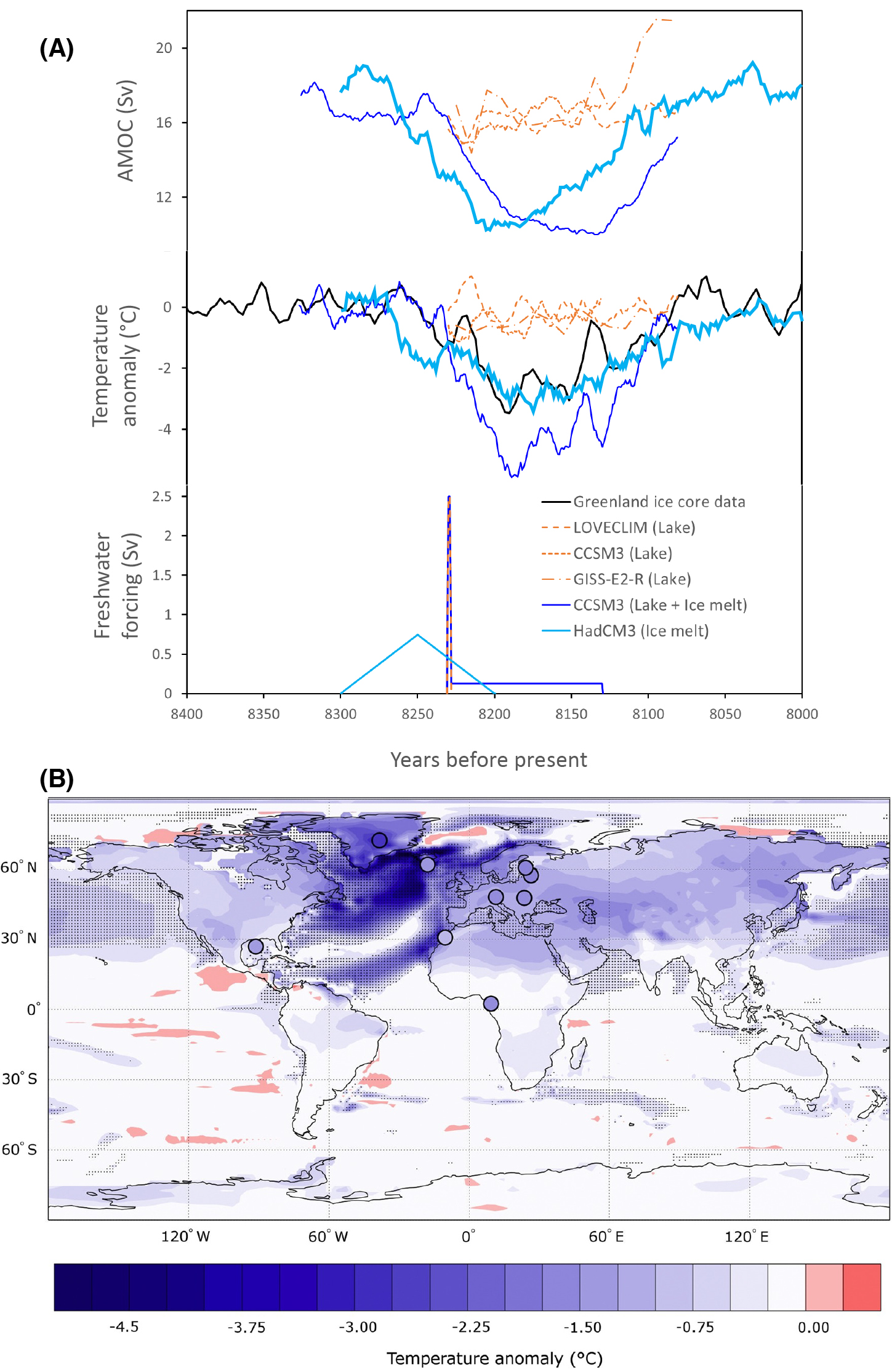
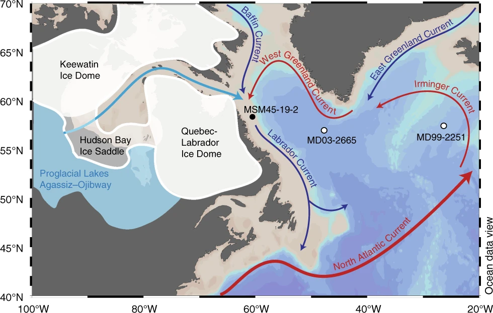
Figure 1: (A) Timeseries of (top) simulated Atlantic Meridional Overturning Circulation, (middle) simulated and observed Greenland temperature, and (bottom) prescribed meltwater forcing from five model experiments of the 8.2 kyr event. Three simulations (orange; Morrill et al. 2013b) that use meltwater fluxes corresponding to the drainage of Lake Agassiz-Ojibway cannot reproduce the duration or magnitude of the event (middle; black), while simulations (blue; Matero et al. 2017; Wagner et al. 2013) that include the much larger and longer ice-melt flux can. (B) The change in annual mean surface temperature caused by an ice-melt flux from the Hudson Bay saddle collapse matches the amplitude of changes in geological records shown in filled circles (reproduced from Matero et al. 2017).

The forcing and mechanism that led to the cooling are now well understood. A release of meltwater into the Labrador Sea freshened sites of deep-water formation, thus slowing the Atlantic Meridional Overturning Circulation (AMOC) and reducing the northward transport of heat in the Atlantic (Barber et al. 1999). Evidence of Labrador Sea freshening and AMOC changes corroborate this story (e.g. Lochte et al. 2019). These changes also coincided with a sudden outburst of the lakes Agassiz and Ojibway (Barber et al. 1999), previously dammed by the remnants of the Laurentide Ice Sheet over North America that was then rapidly retreating (Fig. 2). The lake outburst was thus, for a long time, badged as the culprit for the 8.2 kyr event (Barber et al. 1999).

An ensemble of opportunity

Three climate-modeling groups within PMIP had simulated the event and decided to compare their results for the IPCC Fifth Assessment Report (Morrill et al. 2013b). This exercise was not conducted as a formal model intercomparison project (MIP) as coordinated by PMIP for the mid-Holocene, Last Glacial Maximum, or Pliocene, but was instead an "ensemble of opportunity". The simulations had minor differences in boundary conditions (orbital parameters, greenhouse gases, and ice sheets), but all included a lake outburst freshwater pulse of 2.5 Sv for one year added to the ocean near the Hudson Strait with slight differences in how the water was spread. This volume of freshwater was set to match estimates of lake volume. The models reproduced well the largescale pattern of temperature and precipitation changes deduced from a broad compilation of proxy records (Morrill et al. 2013b). However, the changes caused by the lake outburst were too small and much too short (red lines in Fig. 1), as the slowdown in ocean circulation could not be sustained after the meltwater pulse. Were the models not sensitive enough to this forcing, or was the experimental design inadequate in some way?

'Twas the wrong culprit

Fortunately, the story doesn't end there; it turns out a major factor was missing. The collapse of the Laurentide Ice Sheet that triggered the lake outburst was releasing huge amounts of water in the Labrador Sea and North Atlantic at the time of the event (Gregoire et al. 2012). Sea-level records had shown much larger sea-level rise than what could be explained from the lake outburst (Li et al. 2012), compelling modelers to release more freshwater in their models (Wiersma et al. 2006). It eventually became clear that the melt of the Laurentide Ice Sheet was actually more important than the lake outburst in causing the 8.2 kyr event (Wagner et al. 2013). But why was ice-sheet melt suddenly causing a slowdown of ocean circulation when the ice sheet had been steadily melting for thousands of years?

Figure 2: Map of the Laurentide ice sheet showing the Hudson Bay Ice Saddle that collapsed and the Lakes Agassiz-Ojibway that outburst around the time of the 8.2 kyr event. These caused an influx of freshwater into the Labrador Sea and slowed down the Atlantic Meridional Overturning Circulation causing the cooling shown in Figure 1 (reproduced from Lochte et al. 2019).

The answer came from the discovery of a mechanism of ice-sheet instability, called the saddle collapse, which occurred on two significant occasions during the last deglaciation: one causing the Meltwater Pulse 1a sea-level rise 14.5 thousand years ago, and the other causing the 8.2 kyr event (Gregoire et al. 2012; Matero et al. 2017). The instability occurs during deglaciations when two domes of an ice sheet, connected via an ice saddle, separate to form distinct ice sheets. The saddle collapse is triggered when warming induces melt in the saddle region. As the saddle melts, it lowers, reaching increasingly warmer altitudes, thus accelerating the melt through the ice-elevation feedback, which produces a pulse of meltwater lasting multiple centuries (Gregoire et al. 2012). This is what happened to the ice sheet that was covering the Hudson Bay at the end of the last deglaciation (Gregoire et al. 2012), a process that was possibly enhanced by heat transported from a warm ocean current (Lochte et al. 2019) and instability of the marine parts of the ice sheet (Matero et al. 2020).

Ice collapse and lake outburst

It is not a coincidence that the Lake Agassiz-Ojibway outburst and the Hudson Bay ice-saddle collapse occurred around the same time. Around the peak of the saddle collapse melt, when the ice saddle became thin enough, the lake was able to initiate its discharge via channels under the ice due to the pressure of the lake that sat hundreds of meters above sea level. The ice-sheet melt would have contributed to filling up the lake, and the ice loss likely reduced the gravitational pull that the ice exerted on the ocean and the lake. Thus, estimating the relative timing, amplitude, and location of meltwater discharge from the ice sheet and lake into the ocean requires the combined modeling of the ice-sheet, hydrology, and sea-level processes.

Towards a benchmark for climate sensitivity to freshwater input

Given reasonable scenarios of meltwater discharge into the Labrador Sea from the Hudson Bay saddle collapse, Matero et al. (2017) were able to simulate the duration, magnitude, and pattern of the 8.2 kyr climate changes (Fig. 1, light blue curve), albeit with a larger volume of melt than sea-level records suggest. Our new understanding of the cause of the 8.2 kyr event thus advances the potential of this event to benchmark the sensitivity of climate models to freshwater forcing. Since the event was short and occurred under climate conditions similar to pre-industrial, it could become a feasible "out of sample" target for calibrating climate models. To reach this goal, we must continue to improve estimates for the magnitude, duration, and location of the meltwater forcing by combining sea-level, ocean-sediment, and geomorphological records with models of the ice sheet and lake.

We have good quantitative proxies for circum-North Atlantic temperature change during the event, but additional proxy records in the Southern Hemisphere are needed to determine the extent of the bipolar see-saw, a pattern of southern warming and northern cooling that often occurs when AMOC slows. We also lack good quantitative proxies for precipitation change during the event, which would provide invaluable information on the sensitivity of the water cycle to ice-sheet melt.

The design of MIPs and model–data intercomparison work within PMIP has become highly sophisticated in the last decade with detailed experimental setup for transient climate changes (e.g. DeGLAC; Ivanovic et al. 2016), which include realistic routing of meltwater flux to the ocean. Forward-modeling proxy data such as oxygen isotopes (Aguiar et al. 2021) or ocean neodymium could also greatly improve uncertainty quantification and benchmarking. With all these developments, the 8.2 kyr event may well fulfil its potential as the "Goldilocks" event that could truly test our ability to model the impacts of ice-sheet melting and the response of surface climate to ocean circulation changes.

affiliations

¹School of Earth and Environment, University of Leeds, UK

²University of Colorado and NOAA's National Centers for Environmental Information, Boulder, CO, USA

contact

Lauren J. Gregoire: l.j.gregoireleeds.ac.uk

references

Aguiar W et al. (2021) Sci Rep 11: 5473

Barber DC et al. (1999) Nature 400: 344-348

Gregoire LJ et al. (2012) Nature 487: 219-222

Ivanovic RF et al. (2016) Geosci Model Dev 9: 2563-2587

Lawrence T et al. (2016) Quat Sci Rev 151: 292-308

Li Y-X et al. (2012) Earth Planet Sci Lett 315-316: 41-5

Lochte AA et al. (2019) Nat Commun 10: 586

Matero ISO et al. (2017) Earth Planet Sci Lett 473: 205-214

Matero ISO et al. (2020) Geosci Model Dev 13: 4555-4577

Morrill C et al. (2013a) Clim Past 9: 423-432

Morrill C et al. (2013b) Clim Past 9: 955-968

Schmidt GA et al. (2005) Quat Sci Rev 24: 1109-1110

Wagner AJ et al. (2013) Clim Dyn 41: 2855-2873

Wiersma AP et al. (2006) Clim Dyn 27: 831-849

Chris Brierley¹ and Qiong Zhang²

The midHolocene experiment has been a target period for PMIP activity since the beginning. It has gone through four different iterations in the past 30 years. Over 60 models, of various levels of complexity and resolution, have been used for the midHolocene experiment—contributed from around 20 different modeling groups. They all capture a similar large-scale response, but with a level of detail and understanding that increases with every PMIP phase.

Experimental design

Before describing the design, it is probably worth explaining why the mid-Holocene was chosen as a target period. The ideal period to simulate is one that has a large forced climate change (so a high signal-to-noise ratio), as well as plentiful accurate paleoclimate reconstructions with which to compare the model results. Reconstructions suggest that 6,000 years ago, the tail-end of the African Humid Period, was the warmest portion of the Holocene (COHMAP Members 1988). Yet subsequent transient simulations do not show a warming peak: a "Holocene conundrum" that is not fully resolved (Bader et al. 2020). A different time period might have been chosen today, but the wealth of research focused around 6,000 kyr BP since this period was selected by PMIP means there is little point in deviating now.

The midHolocene experiment has kept the same orbital settings since its inception, although other aspects of the design have evolved over the years (Joussaume and Taylor 1995; Otto-Bliesner et al. 2017). The main forcing is an alteration in the precession by roughly a right angle—6,000 years ago the Earth was closest to the sun in Northern Hemisphere (NH) autumn, not during NH winter as is the case today. Determining a consistent way to apply this change was tricky, because of the way orbits, incoming insolation, and internal model calendars are embedded in model radiative codes. The implications of internal calendars being hardwired in models' data output routines are still being felt and need to be considered in analyses (Bartlein and Shafer 2019). The obliquity and eccentricity are also altered. Other settings, such as land cover and atmospheric composition, follow the standard control simulation (i.e. perpetual 1850 CE conditions, except for PMIP1 which used an atmosphere-only set up). For the first time, PMIP4 applied observed greenhouse gas conditions for 6,000 kyr BP, mainly a drop in CO₂ levels of 25ppm from ∼284 ppm in the pre-industrial (Otto-Bliesner et al. 2017).

Uptake and reach

More models have performed midHolocene simulations than any other PMIP run—mainly due to the relative ease of prescribing its boundary conditions. The headline papers of the four different PMIP phases include a total of 60 models (Joussaume et al. 1999; Braconnot et al. 2007; Braconnot et al. 2012; Brierley et al. 2020); further, models have performed this standard experiment outside of those publications. There has been a steady increase in both model resolution and complexity throughout the four phases (Braconnot et al. this issue). The simulations have gained models of the ocean, sea ice, and increasingly interactive vegetation. This latter component helps with the expansion of the North African monsoon into the "green Sahara", but models still do not fully capture this transition (Brierley et al. 2020).

There have been a large number of researchers involved with the PMIP midHolocene simulations, with 77 different authors on the four initial description papers alone. Many publications have been written (nearly 2,000 that include PMIP and mid-Holocene in their keywords), and this number will only increase with time. The midHolocene experiment has also been discussed in all IPCC reports since AR3 (Kageyama et al. this issue, p. 68).

Findings

The midHolocene experiment reassuringly demonstrates that climate models show a consistent response to changes in radiative forcings that fits well with our theoretical understanding of the Earth system. The shift in the seasonal distribution of incoming solar energy leads to seasonal temperature changes that are amplified by continentality. These temperature changes lead to variations in the thermal equator and hence the seasonal march of the intertropical convergence zone (ITCZ) and the associated precipitation patterns. These fundamental features of mid-Holocene climate are found in paleoclimate reconstructions and have been present in results from simulations since PMIP1 (Joussaume et al. 1999).

The creation of ensembles of simulations focused at 6,000 years ago has spurred concerted efforts within the paleoclimate data community. It has motivated researchers to include the period when designing the creation of individual reconstructions. There is a dimensional difference between model simulations, which have global spatial coverage for a limited time, and paleoclimate reconstructions, which track time variations at a fixed location. Data compilations from a time-slice centered on the mid-Holocene have been created to overcome this (Bartlein and Webb, this issue). These compilations also permit the quantitative benchmarking of the midHolocene simulations (Harrison et al. 2014). Although this remains challenging to undertake, results have contributed to IPCC assessments of models (Kageyama et al. this issue, p. 68).

Paleoclimate compilations highlight the dramatic changes in hydroclimate that happened during the mid-Holocene in the subtropics. The African Humid Period, colloquially called the "green Sahara", is associated with a dramatic poleward extension of the West African monsoon and wetter conditions across northern Africa. It started prior to the Holocene and had already ended in some locations by 6,000 years ago (Shanahan et al. 2015). This has been a focus of analysis since the first phase of PMIP (Joussaume and Taylor, this issue; Braconnot et al. this issue).

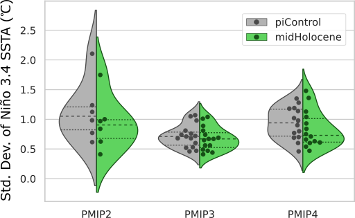Figure 1: ENSO activity, as measured by the standard deviation of monthly sea surface temperature anomalies averaged over the "Niño 3.4" region of the equatorial Pacific, in PMIP2 (An and Choi 2014), PMIP3, and PMIP4 (Brown et al. 2020).

Around the time of the completion of PMIP1 came the discovery that ENSO variability in reconstructions was weaker during the mid-Holocene (Rodbell et al. 1999). This opened a new possible research avenue (Rehfeld and Brown, this issue), which has now become a major focus of activity around the midHolocene simulations (Zheng et al. 2008; An and Choi 2014; Brown et al. 2020). Models show reduced ENSO activity in response to the mid-Holocene orbital changes. Over the three PMIP phases with coupled models (PMIP2–PMIP4), the ENSO reduction has become more consistent (Fig. 1). Yet the mechanisms for this response are not entirely clear, complicating our ability to pull that success forward into more confident projections of future ENSO changes.

Outside of the tropics, the results of the midHolocene experiment show large seasonal temperature variations. One consequence of this is a reduction in summer sea-ice extent in the Arctic (Fig. 2). Non-linear feedbacks of both this and the increase in winter sea ice result in increasing uncertainty regarding the annual mean temperature change in the Arctic. There is however a robust relationship between Arctic temperature change and sea-ice extent in the models, which seems more consistent in PMIP4 compared to earlier phases.

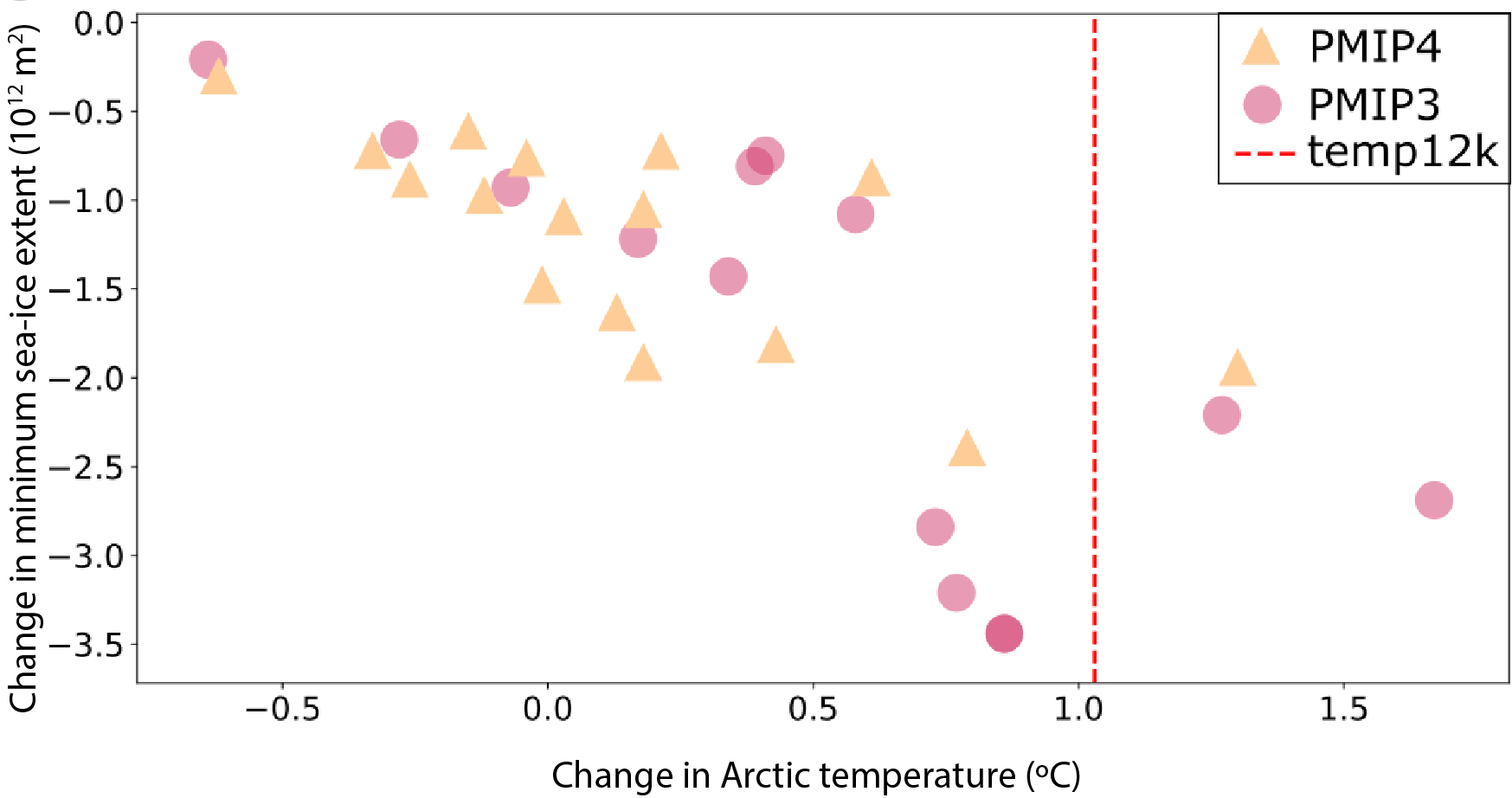Figure 2: The relationship between the change in annual mean Arctic temperatures and the Northern Hemisphere minimum sea-ice extent (Brierley et al. 2020). The median of the annual mean temperature changes over the Arctic reconstructed by the Temperature 12k compilation of Kaufman et al. (2020) is shown as a vertical line.

Outlook

The ensemble of PMIP4 midHolocene simulations has only recently been completed, and publications documenting the individual constituent simulations are still emerging. We envisage that the midHolocene simulations will be the focus of many multi-model analyses in the next couple of years. The PMIP structure, part of a global modeling effort that includes future scenarios, permits these analyses to readily include multiple experiments. The combination with the lig127k experiment (Otto-Bliesner et al. this issue) allows the robustness and magnitude of orbital forcing to be assessed. The combination with warming experiments, be they either idealized simulations or future scenarios, allows the lessons from the mid-Holocene to be quantitatively connected to the associated changes anticipated for this century. Personally, we would love to see greater use of the midHolocene simulations amongst the wider climate modeling community, for example by working together with the global monsoon MIP or sea-ice MIP efforts.

Finally, it is worth asking whether the next generation of coupled models should also run midHolocene experiments. We are now in the position where transient Holocene simulations with GCMs are feasible (Otto-Bliesner et al. 2017). These are more intellectually stimulating, remove some problems with data–model comparisons, and perhaps are more helpful for future scenarios (which themselves are mostly transient). However, Holocene transients cannot be made with the shiniest, most computationally expensive models. Over the next few years of analyses on the PMIP4 midHolocene simulations, we must investigate whether the effort and resources needed to use the state-of-the-art models are justifiable, for example, by exploring the experiment's potential to evaluate interactive vegetation, dust, and carbon cycle models.

affiliations

¹Department of Geography, University College London, UK

²Department of Physical Geography, Stockholm University, Sweden

contact

Chris Brierley: c.brierleyucl.ac.uk

references

An S-I, Choi J (2014) Clim Dyn 43: 957-970

Bader J et al. (2020) Nat Commun 11: 4726

Bartlein PJ, Shafer SL (2019) Geosci Model Dev 12: 3889-3913

Braconnot P et al. (2007) Clim Past 3: 261-277

Braconnot P et al. (2012) Nat Clim Chang 2: 417-424

Brierley CM et al. (2020) Clim Past 16: 1847-1872

Brown JR et al. (2020) Clim Past 16: 1777-1805

COHMAP Members (1988) Science 241: 1043-1052

Harrison SP et al. (2014) Clim Dyn 43: 671-688

Joussaume S, Taylor KE (1995) Status of the paleoclimate modeling intercomparison project, Proceedings of the first international AMIP scientific conference, WCRP Report, 425-430

Joussaume S et al. (1999) Geophys Res Lett 26: 859-862

Kaufman D et al. (2020) Sci Data 7: 201

Otto-Bliesner BL et al. (2017) Geosci Model Dev 10: 3979-4003

Rodbell DT et al. (1999) Science 283: 516-520

Shanahan T et al. (2015) Nat Geosci 8: 140-144

Zheng W et al. (2008) Clim Dyn 30: 745-762

Johann H. Jungclaus¹, O. Bothe², E. Garcia-Bustamante³, J.F. González-Rouco⁴, R. Neukom⁵ and A. Schurer⁶

Simulations of Common Era climate evolution coordinated by PMIP's "Past2K" working group together with multi-proxy reconstructions from the PAGES 2k Network provide pivotal understanding for the evolution of the modern climate system and for expected changes in the near future.

Transient simulations of the recent past

Knowledge of past climate evolution is essential for understanding natural variability and for providing context for current and future climate change. One example is the Common Era (CE, i.e. approximately the last 2000 years) with its vast collection of proxy, observational, and documentary datasets, which often feature annual or sub-annual resolution. Simulations covering the CE or the last millennium (LM, i.e. the 1000 years before the industrial era, 850 to 1850 CE) are essential to identify plausible mechanisms underlying paleoclimatic observations and reconstructions. Applying the same models to study past, present, and future climate and its response to external forcing enables the community to use paleodata for the evaluation of the Earth system models that we use for climate projections.

Looking back at more than 20 years of progress in the simulation of CE climate evolution, success of these experiments rests on three pillars: (1) models suitable for a realistic representation of regional and global variability and with an adequate response behavior to external forcing agents; (2) reliable estimates of external forcing factors, such as solar irradiance or volcanic sulfur injections; and (3) the availability of reliable observational or proxy-based reconstructions for model–data comparison.

Simulating 1000 years or even longer periods is challenging in terms of computational resources. Early approaches to simulate the LM have therefore applied simplified models, such as energy-balance models (Crowley 2000), or models of intermediate complexity (Goosse et al. 2005). However, starting already in the late 1990s, millennium-long simulations using comprehensive ocean-atmosphere general circulation models (like the legendary "Erik" runs; González-Rouco et al. 2003) paved the way for more complex analyses of dynamical changes and regional climate variations. Over the first decade of the 21st century, more modeling groups became interested in LM simulations (see Fernandez-Donado et al. 2013 for a review), and progress in model development allowed for more complexity to be included, for example the interactive simulation of the carbon cycle (Jungclaus et al. 2010) or ozone chemistry (Shindell et al. 2001).

Last millennium simulations in PMIP3/CMIP5

Considering the role of information from paleoarchives and modeling in the Intergovernmental Panel on Climate Change (IPCC) assessment reports (AR), the PMIP workshop in Estes Park, USA, in 2008 (Otto-Bliesner et al. 2009) suggested that coordinated simulations of the LM should receive high priority in PMIP's contribution to the fifth phase of the Coupled Model Intercomparison Project (CMIP5). Consequently, a working group was established to coordinate the experiments and to discuss a common basis for "past1000" simulations covering the period 850 to 1850 CE. Schmidt et al. (2011) provided a comprehensive protocol on which modeling groups were able to build their experimental strategy. Additionally, the adaptation of the CMIP5 data format conventions facilitated the distribution of data through CMIP's Earth System Grid Federation framework. The initiative resulted in contributions from 10 modeling groups, including institutions that were previously not active in PMIP. Several of those provided multiple realizations or sensitivity experiments using, for example, different flavors of solar forcing (Masson-Delmotte et al. 2013, Fig. 5.8).

PMIP and PAGES2k collaboration and scientific achievements

The endorsement of the LM simulation as a key experiment in PMIP coincided with the launch of the Past Global Changes PAGES 2k Network (PAGES2k; pastglobalchanges.org/2k) in 2008. Consequently, both initiatives have collaborated and profited from each other. Common work on reconstruction and model simulations was reflected at prominent places in IPCC's AR5 (Masson-Delmotte et al. 2013). For example, based on the comparison between reconstructions and simulations, the authors of AR5 concluded that there is high confidence that not only external orbital, solar, and volcanic forcing but also internal variability contributed substantially to the spatial pattern and timing of surface temperature changes between the Medieval Climate Anomaly and the Little Ice Age. The AR5 also highlighted significant differences between unforced and forced "past1000" simulations that can be identified on timescales larger than 50 years, indicating the importance of forced variability on these timescales.

The first phase of PAGES2k had a focus on regional temperature reconstructions, and a community-building workshop was held in 2013 in Madrid. The workshop led to the initiation of assessments of regional temperature responses to external forcing, and the PAGES2k-PMIP3 group (2015) concluded that the response to external forcing is detectable in the Northern Hemisphere during all time periods over the last 2000 years (Fig. 1). The role of solar forcing was investigated and found to be comparatively smaller than that of the volcanic forcing. Data–model agreement was considerably lower in regions in the Southern Hemisphere compared to the Northern Hemisphere. To understand these still substantial differences over large parts of the globe, improved proxy data coverage and understanding of dynamical processes, such as variability modes, was identified as a priority for future work.

Figure 1: Detection and attribution results for regions defined by PAGES Hydro2k Consortium (2017). Scaling factors (bars, 5-95% range) significantly offset from "0" indicate that the response to forcing is detected, and those that encompass "1" indicate that the magnitude of the forced response agrees with simulations. A circle indicates that the detection analysis was successful, namely the forced response is significantly greater than zero and a residual consistency check was passed (modified from PAGES2k-PMIP3 group 2015).

Moving beyond temperature reconstructions and to the second phase of PAGES2k, another workshop at the Lamont-Doherty Earth Observatory in the Palisades, USA, in 2016 (pastglobalchanges.org/calendar/26535) concentrated on hydroclimatic aspects and refined best practices for model–data comparisons of hydroclimate over the CE (PAGES Hydro2k Consortium 2017). The workshop also covered novel aspects such as proxy system modeling and the interactive simulations of water isotopes as it is promoted in PAGES2k's Iso2k project (pastglobalchanges.org/iso2k).

For other PAGES2k initiatives, for example those working on sub-continental temperature reconstructions, the "past1000" multi-model ensemble was instrumental in understanding the mechanisms driving global and regional climate variability on interannual to centennial timescales. For example, Neukom et al. (2019) confirmed the lack of preindustrial spatial coherence in temperature both in field reconstructions and LM simulations (Fig. 2).

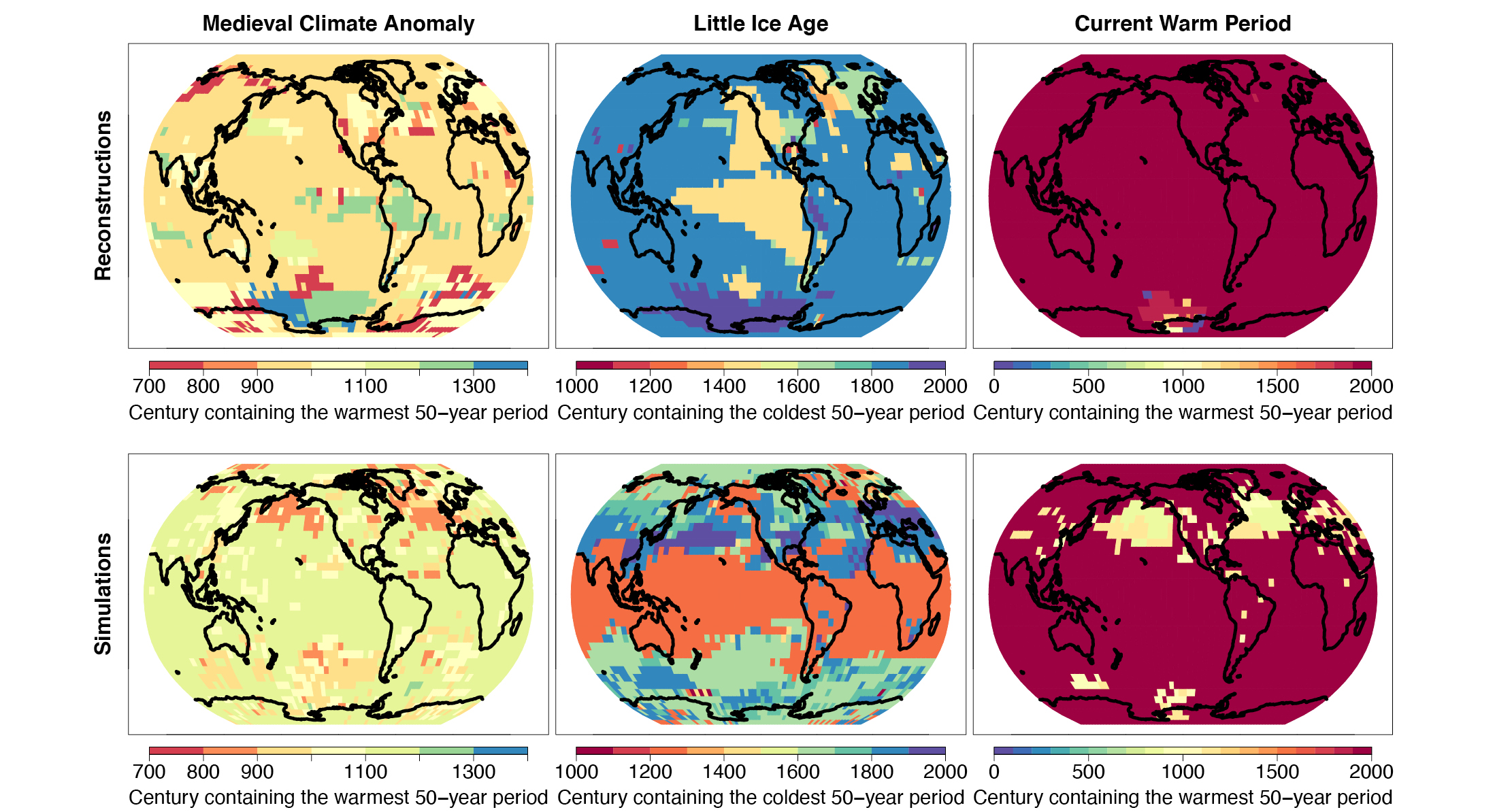Figure 2: Spatially resolved temperature reconstructions (upper row) and corresponding model simulations (lower row) demonstrate that warm and cold periods prior to the current warm period were not globally synchronous (modified from Neukom et al. 2019).

From PMIP3 to PMIP4

Preparing for the sixth phase of CMIP (CMIP6), the PMIP community designed experiments for five different periods. Among others, this included the LM, in order to address the CMIP science objectives defined by the World Climate Research Program. Fostering proper model documentation, CMIP6 introduced a new structure, where a set of common standardized experiments (e.g. idealized CO₂-increase experiments) is accompanied by CMIP-endorsed experiments, like PMIP. The experimental protocol for CE simulations (Jungclaus et al. 2017) reflected refinements in the external forcing agents, in particular solar irradiance, volcanic forcing, and land-cover/land-use changes. The protocol adopted CMIP's "tiered" structure to prioritize certain simulations, e.g. requiring an experiment with an agreed-on standard forcing. The protocol allowed for innovations such as interactive aerosol modules requiring volcanic emissions rather than optical properties to be included. Modeling groups were also encouraged to provide multiple realizations of single-forcing sensitivity experiments, or to expand the temporal range of simulations to include the entire CE. Another novel aspect seen in CMIP6 is that more models include additional features, such as interactive simulation of water isotopes (e.g. Brady et al. 2019).

During the CMIP6 preparation and production phase, PMIP groups concentrated on modeling aspects; now, the new PMIP4/CMIP6 simulations are just about to be harvested by the community. For example, the first "Past2K" simulation was analyzed with a focus on the volcanically active 6th century (Van Dijk et al. 2021).

Moreover, remarkable progress was achieved by individual groups and consortia outside the PMIP working group. We name here in particular the "Last Millennium Ensemble" (LME) project by NCAR (Otto-Bliesner et al. 2016), data assimilation (DA), and DA-based reconstruction (e.g. the "Last Millennium Reanalysis Project"; Hakim et al. 2016), and DA including the reconstruction of hydroclimate (Steiger et al. 2018).

At the same time, PAGES2k is moving into its fourth phase, which will begin at the start of 2022. Community consultation so far has indicated particular interest in hydroclimate, regional and large-scale climate process, data–model integration, and proxy system modeling. Thus, given the progress in modeling during the CMIP6 phase, for example the availability of simulations over the entire CE or more isotope-enabled models, the 30-year anniversary of PAGES and PMIP appears to be an excellent time, in particular for early-career scientists, to continue cooperative research on the climate of the Common Era.

affiliations

¹Max Planck Institute for Meteorology, Hamburg, Germany

²Helmholtz-Zentrum Hereon, Geesthacht, Germany

³Centro de Investigaciones Energéticas, Medioambientales y Tecnológicas, Madrid, Spain

⁴Department of Earth Physics and Astrophysics, Geosciences Institute IGEO (UCM-CSIC), Complutense University of Madrid, Spain

⁵Department of Geography, University of Zurich, and Department of Geosciences, University of Fribourg, Switzerland

⁶School of Geosciences, University of Edinburgh, UK

contact

Johann Jungclaus: johann.jungclausmpimet.mpg.de

references

Brady E et al. (2019) J Adv Model Earth Syst 11: 2547-2566

Crowley TJ (2000) Science 289: 270-277

Fernandez-Donado L et al. (2013) Clim Past 9: 393-421

Goosse H et al. (2005) Quat Sci Rev 24: 1345-1360

González-Rouco JF et al. (2003) Geophys Res Lett 30: 2116

Hakim GJ et al. (2016) J Geophys Res Atmos 121: 6745-6764

Jungclaus JH et al. (2010) Clim Past 6: 723-737

Jungclaus JH et al. (2017) Geosci Model Dev 10: 4005-4033

Masson-Delmotte V et al. (2013) In: Stocker TF et al. (Eds) Climate Change 2013: The Physical Science Basis. Cambridge University Press, 383-464

Neukom R et al. (2019) Nature 571: 550-554

PAGES Hydro2k Consortium (2017) Clim Past 13: 1851-1900

PAGES2k-PMIP3 group (2015) Clim Past 11: 1673-1699

Otto-Bliesner BL et al. (2009) Eos 90: 11

Otto-Bliesner BL et al. (2016) Bull Am Meteorol Soc 97: 735-754

Schmidt GA et al. (2011) Geosci Model Dev 4: 33-45

Shindell DT et al. (2001) Science 294: 2149-2152

Steiger N et al. (2018) Sci Data 5: 180086

Van Dijk E et al. (2021) Clim Past Discuss, doi:10.5194/cp-2021-49

Patrick J. Bartlein¹ and Thompson Webb III²

Syntheses of terrestrial paleoclimatic data have a long history, but in the 1980s they rapidly developed into the database-in-a-repository form we know today. Over time they have anchored the productive interaction with climate-model simulations aimed at both testing the models and explaining patterns in the data.

One of the basic tasks of PMIP (and its predecessor studies) is the comparison of climate-model simulations with paleoenvironmental observations. This is motivated by the dual objectives of using the observations to "benchmark" or test the models, and using the physically based models to provide mechanistic explanations for the observed patterns in the data (Braconnot et al. 2012; Harrison et al. 2015). These objectives have in turn motivated the synthesis of paleoenvironmental data from both terrestrial and marine sources and their interpretation. Here we review some of the past terrestrial syntheses, and their evolution over time.

Early syntheses

Before the mid-1970s, syntheses of terrestrial paleoenvironmental data were available in book form, as textbooks (e.g. Brooks 1949; Zeuner 1959; Frenzel 1967; and R.F. Flint's evolving sequence: 1947, 1957, and 1971), edited volumes (e.g. Nairn 1961; Wright and Frey 1965), and H.H. Lamb's (1971, 1977) two-volume treatise. Although not databases in any sense, such publications were the places to go for broad descriptions of past climates and the observations they were based on.

Also of note from this era was a U.S. National Academy of Sciences report, Understanding Climatic Change, prepared by the U.S. Committee for the Global Atmospheric Research Program (USCGARP 1975). This study included Appendix A, a survey of past climates by Imbrie, Broecker, Mitchell, and Kutzbach, that included some temporal and spatial syntheses of climatic variations. Many of the themes and proposals for climate-research action discussed there (such as the joint elaboration of paleoclimatic databases and development of simulation models of both present and past climates) would seem familiar today.

CLIMAP era

CLIMAP (Climate: Long range Investigation, Mapping, and Prediction) was a collaborative project aimed at reconstructing conditions at the Last Glacial Maximum, in particular the distribution of ice sheets, seasonal sea-surface temperatures, and land-surface albedo. The main results of the reconstructions appeared in Science (CLIMAP Project Members 1976), and more fully in an edited volume (Cline and Hays 1976), and a set of maps (CLIMAP Project Members 1981). In a companion paper, Gates (1976) described the results of a GCM simulation with surface boundary conditions provided by the CLIMAP reconstructions. Although not the first attempt at paleo simulation, the paper did feature what might be regarded as a canonical mode of data–model comparison—dots on a map.

Running through the CLIMAP-era discussions was the notion that if the goal was comparison of paleo-observations and climate-model simulations, then more paleo-data were surely needed. This began to be realized late in the 1970s. For example, Bernabo and Webb (1977) described mapped summaries of Holocene pollen data from northeastern North America, and similar work was underway for Europe (Huntley and Birks 1983). A special issue of Quaternary Research (Hecht et al. 1979) contained the first really comprehensive syntheses of terrestrial paleoclimatic data on a global scale (Peterson et al. 1979; Street and Grove 1979).

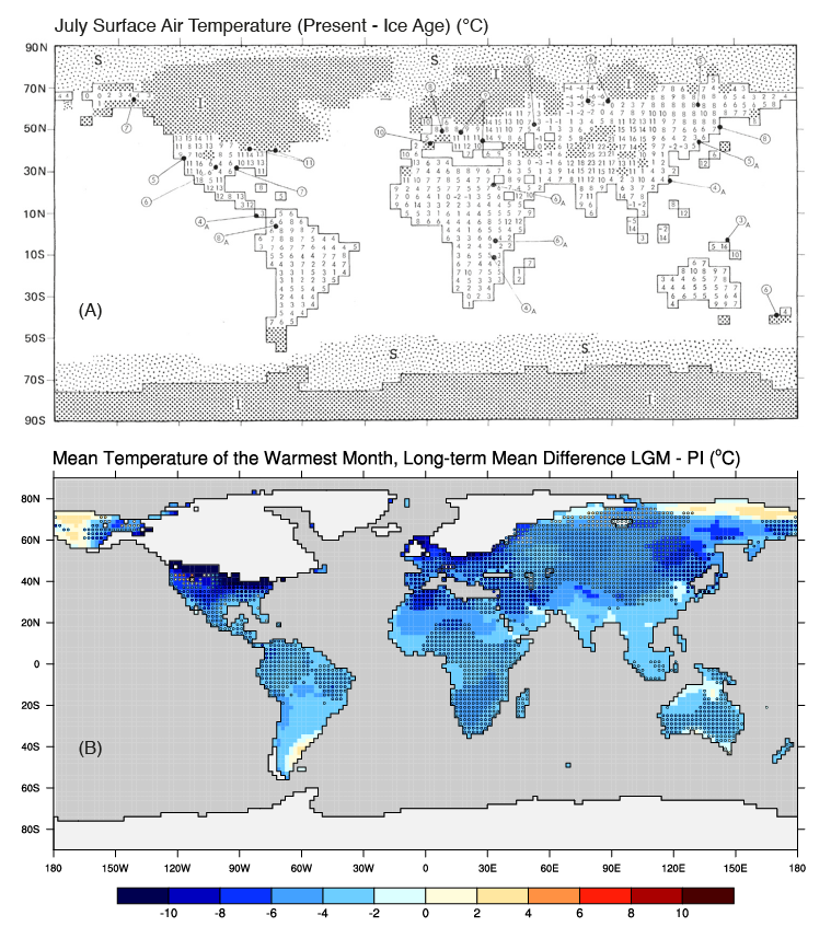Figure 1: Forty-five years of progress in terrestrial data–model comparisons. (A) CLIMAP-era comparisons of simulated (values on the model grid) and reconstructed (circles and dots) July temperature difference (present-day minus ice age); figure modified from Gates (1976). (B) Gridded reconstructions of the Last Glacial Maximum minus present mean temperature of the warmest month (colored dots, data from Cleator et al. 2020), plotted over CMIP5/PMIP3 lgm – piControl multi-model means on a 2-degree grid (see Harrison et al. 2014).

Peterson et al. (1979) brought together data for the LGM, and introduced the notion of "levels of analysis of the data: I: "raw" pollen, lake-level, etc. data; II: Level I data converted to estimates of specific climatic variables; and III: Level II data combined from various sources, and interpolated and contoured. (From a data-preservation perspective, we might now consider a Level 0—the materials themselves, e.g. Palmer et al. 2021, and Level IV—coordinated data sets of multiple kinds of data linked to one another, Grobe et al. 2021). Peterson et al. also addressed chronological uncertainties, introducing a three-level classification (later refined to seven levels by Webb 1985a), and the question of how much data is enough for valid comparisons. Street and Grove (1979) described lake-status data both temporally and spatially over the past 30 kyr. The syntheses were not electronic, and the results exist today only as .pdfs of the articles. However, they contained data-availability statements, perhaps some of the earliest. The 150-page Appendix to Peterson et al. could be obtained for the price of photocopying (probably ∼USD 7.50), while the Street and Grove data would be furnished on microfiche for USD 2.50.

COHMAP era

COHMAP (Cooperative Holocene Mapping Project; Wright et al. 1993; Wright and Bartlein 1993) was an international, interdisciplinary research group that became organized in the late 1970s, benefiting from the experiences of several of the participants in CLIMAP. The project evolved to focus on a suite of paleoclimatic simulations at 3-kyr intervals from the Last Glacial Maximum to present, and parallel syntheses of terrestrial and marine data and climate reconstructions based on them (e.g. COHMAP Members 1988).

By 1980, it became obvious that photocopy and microfiche distribution was not ideal. Personal computers were becoming widely available as were connections to the forerunners of the internet, and this pushed along the electronic distribution of data.

What might be regarded as the first "modern" syntheses were a global compilation of the climate of 6000 yr BP and the supporting data (Webb 1985a) and a synthesis of lake-level status for the COHMAP target times (Street-Perrott et al. 1989). These studies had both printed and electronic components (on magnetic tape), and remarkably, the .pdfs of the printed reports and the data files are still available online. The collections of individual files are easily recognizable as the elements of a relational database, and feature such components of 21st-century databases as "rich" site metadata, separation of the chronologies or age models from the data, adoption of common vocabularies, harmonization of taxa, sediments, depositional environments, and links to publications and to the data originators.

The databases of that era represented snapshots of data available at the time of publication, and, unlike today, there was no provision for updating. This led to another strategy for database development that is still in use today: a distinction between a database (in a repository) and a "research data set", which may include newer published and unpublished data. The published databases, along with continuously updated research data sets, supported analysis of the data (e.g. Webb 1985b; Street-Perrott and Harrison 1985; COHMAP Members 1988; Harrison 1989).

PMIP era

By the mid 1990s, databases of the 1980s were being regularly elaborated and enlarged, while contributing to the evaluation of newer sequences of climate-model experiments (e.g. Webb and Kutzbach 1998) and to the first generation of PMIP experiments (Joussaume et al. 1999). Examples include lake-status records for Europe and elsewhere produced by Sandy Harrison and associates, often published as a journal article and companion data release (e.g. Yu and Harrison 1995a; 1995b) – anticipating the current FAIR Principles for data management and stewardship. Pollen databases were organized for each continent (e.g. NAPD and EPD, the North American and European Pollen Database(s), Grimm et al. 2018 provides a history). The pollen databases contributed to Level III-type syntheses, such as that represented by the reconstruction of vegetation at 6000 yr BP and the LGM (Prentice and Webb 1998; Boenisch et al. 2001).

Over the past decade, databases or syntheses that contribute to the design or evaluation of the current (PMIP4) generation of simulations came online, including those for standard and "deep-time" experiments (e.g. Cleator et al. 2020; Hollis et al. 2019; Dowsett et al. 2016), as well as those for the last millennium, such as the International Tree-Ring Data Bank (Zhao et al. 2018) and the PAGES2k Consortium (2013; 2017) database of temperature reconstructions. Other databases that have yet to "fully participate" in PMIP-style data–model comparisons include those for biomass burning and paleofire (Marlon et al. 2016) and speleothem isotopes (Comas-Bru et al. 2020). Recently "databases of databases" have appeared including the Neotoma Paleoecology Database (Williams et al. 2018b; Grimm et al. 2018), which folded in many earlier paleoecological-focused efforts and greatly expanded the content and usability of the data.

Today the amount of data has begun to impact their usability (Khider et al. 2019), and external (to PMIP or to paleoclimatology in general) demands on paleoscience require answering more complicated questions than "What happened?" or "Do the models really work?" Those issues are being addressed; see, for example, the November 2018 issue of Past Global Changes Magazine (Williams et al. 2018a) and Grobe et al. (2021).

One common theme in the history of syntheses of terrestrial paleoclimatic data is the goal of making the data available, whether via book, edited volume, multiple-authored article, or adopted new technologies. A second common theme is the continuous interaction between scientific questions and data availability. Hypotheses about how the climate system works, expressed either as predictions from conceptual models or output from climate-model simulations, demand data for testing. The patterns in the data, both temporal and spatial, demand explanation and in turn generate new questions and hypotheses. That interaction between the data and models makes the intellectual environment of paleoclimatology rich and motivates continued data generation, curation, and synthesis.

affiliations

¹Department of Geography, University of Oregon, Eugene, OR, USA

²Department of Earth, Environmental and Planetary Sciences, Brown University, Providence, RI, USA

contact

Pat Bartlein: bartleinuoregon.edu

references

Bernabo JC, Webb T III (1977) Quat Res 8: 64-96

Boenisch G et al. (2001) BIOME 6000 Data Release 1, IGBP PAGES/World Data Center for Paleoclimatology Data Contribution Series # 2001-046. NOAA/NGDC Paleoclimatology Program, Boulder, CO, USA

Braconnot P et al. (2012) Nat Clim Change 2: 417-424

Brooks CEP (1949) Climate Through the Ages, Rev Ed. McGraw-Hill, 395 pp Cleator SF et al. (2020) Clim Past 16: 699-712

Data: doi.org/10.17864/1947.244

CLIMAP Project Members (1981) Seasonal reconstruction of the Earth's surface at the last glacial maximum. Geol Soc Am, Map and Chart Series, pp 1-18

Digital data: ncdc.noaa.gov/paleo-search/study/2516

PDFs of the maps: rock.geosociety.org/Store/detail.aspx?id=MCH036P

Cline RM, JD Hays (1976) Geol Soc Am Memoirs 145

COHMAP Members (1988) Science 241: 1043-105

Comas-Bru L et al. (2020) Earth Syst Sci Data 12: 2579-2606

Data: doi.org/10.17864/1947.256

Dowsett H et al. (2016) Clim Past 12: 1519-1538

Flint RF (1947) Glacial Geology and the Pleistocene Epoch. Wiley, 589 pp

Flint RF (1957) Glacial and Pleistocene Geology. Wiley, 553 pp

Flint RF (1971) Glacial and Quaternary Geology. Wiley, 892 pp

Frenzel B (1967) Die Klimaschwankungen des Eiszeitalters. Vieweg+Teubner Verlag, 244 pp

Gates WL (1976) Science 191: 1138-1144

Grimm EC et al. (2018) PAGES Mag 26: 64-65

Grobe H et al. (Eds; 2021) Paleoclimate data synthesis and analysis of associated uncertainty. Special issue jointly organized between Biogeosci, Clim Past, and Earth Syst Sci Data

Harrison SP (1989) Clim Dyn 3: 157-167

Harrison SP et al. (2014) Clim Dyn 43: 671-688

Harrison SP et al. (2015) Nat Clim Change 8: 735-743

Hecht AD et al. (1979) Quat Res 12: 6-17

Hollis C et al. (2019) Geosci Model Dev 12: 3149-3206

Huntley B, Birks HJB (1983) An Atlas of Past and Present Pollen Maps for Europe, 0-13,000 years ago. Cambridge University Press, 667 pp

Joussaume S et al. (1999) Geophy Res Let 27: 859-862

Khider D et al. (2019) Paleoceanogr Paleoclimatol 34: 1570-1596

Lamb HH (1971) Climate: Present, Past and Future. Volume 1: Fundamentals and Climate Now. Methuen/Routledge, 613 pp

Lamb HH (1977) Climate: Present, Past and Future. Volume 2: Climatic History and the Future. Methuen/Routledge, 870 pp

Marlon JR et al. (2016) Biogeosci 13: 3225-3244 data available at: https://paleofire.org

Nairn AEM (1961) Descriptive Paleoclimatology. Interscience, 380 pp

PAGES2k Consortium (2013) Nat Geosci 6:339-346

PAGES2k Consortium (2017) Sci Data 4: 170088

Palmer J (2021) Eos 102: 22-29

Peterson GM et al (1979) Quat Res 12: 47-82

Prentice IC, Webb T III (1998) J Biogeogr 25: 997-1005

Street FA, Grove AT (1979) Quat Res 12:83-118

Street-Perrott FA, Harrison SP (1985) In: Hecht AD (Ed) Paleoclimate Analysis and Modeling. Wiley, 291-340

Street-Perrott FA et al. (1989) Global Lake-Level Variations from 18,000 to 0 Years Ago: A Paleoclimatic Analysis. U.S. Department of Energy Technical Report 46, Washington, D.C. 20545. Available from the National Oceanic and Atmospheric Administration, National Center for Environmental Information ("NOAA Paleo")

USCGARP (United States Committee for the Global Atmospheric Research Program) (1975) Understanding Climatic Change.

Webb T III (1985a) Global Paleoclimatic Data for 6000 Yr B.P. U.S. Department of Energy Technical Report 18, Washington, D.C. 20545. Available from the U.S. Department of Energy, Office of Scientific and Technical Information: osti.gov/search/semantic:10.3334/CDIAC/cli.ndp011

Webb T III (1985b) In: Hecht AD (Ed) Paleoclimate Analysis and Modeling. Wiley, 163-195

Webb T III, Kutzbach JE (1998) Quat Sci Rev 17: 465-471

Williams JW et al. (2018a) PAGES Mag 26: 49

Williams JW et al. (2018b) Quat Res 89: 156-177

Wright HE Jr, Frey DG (Eds; 1965) The Quaternary of the United States. Princeton University Press 922 pp

Wright HE Jr. et al. (Eds; 1993) Global Climates since the Last Glacial Maximum. University Minnesota Press, 569 pp (see Preface and Introduction)

Wright HE Jr, Bartlein PJ (1993) Holocene 3: 89-92

Yu G, Harrison SP (1995a) Boreas 24: 260-268

Yu G, Harrison SP (1995b) Lake status records from Europe: Data base documentation IGBP PAGES/World Data Center-A for Paleoclimatology Data Contribution Series # 95-009 NOAA/NGDC Paleoclimatology Program, Boulder, CO, USA

Zeuner FE (1959) The Pleistocene Period: Its Climate, Chronology and Faunal Successions. Hutchinson Scientific & Technical, 447 pp

Zhao S et al. (2018) J Beogeog 46: 355-368

Data: ncdc.noaa.gov/data-access/paleoclimatology-data/datasets/tree-ring