PAGES Magazine articles

Antti E.K. Ojala1, C. Bigler2 and J. Weckström3

Sediment trapping and monitoring is essential for paleolimnological research. It has allowed us to understand the seasonal deposition of the abiotic and biotic components within varved lakes in Sweden and Finland, thus providing a basis for paleoenvironmental interpretations.

Varved sediments are rich and detailed archives of paleoenvironmental information. Interpreting these archives correctly requires that the sedimentological processes leading to the varve deposition and their controlling factors are known, understood and quantified. Modern lake research, particularly when dealing with seasonally to annually resolved varved sediments, combines limnological monitoring, sediment trapping and sediment analysis (Leemann and Niessen 1994; Bigler et al. 2012; Ojala et al. 2013). The reason for such an integrative approach is to understand to what extent the sediments and its components reflect the ongoing sedimentary and biogeochemical processes within a lake basin (Ryves et al. 2013). Monitoring and trap studies also enable us to better understand the seasonal information within a varve (i.e. definition of a local varve model) and effectively calibrate varves and paleolimnological proxies against instrumental hydrological and meteorological data.

Varve formation

For proglacial lakes with clastic varves (Leemann and Niessen 1994; Lamoureux 1999) and Boreal lakes with clastic-biogenic varves (Renberg 1982; Zillén et al. 2003; Ojala et al. 2000), the deposition of varves is a function of hydrometeorological parameters, in particular seasonal runoff and the associated discharge of suspended sediment from the catchment into the depositional basin. However, as discussed by Lamoureux (2012), the deposition of allochthonous clastic material is also affected by limnological and geomorphological features, which determine sediment pathways to deposition and the yield from the catchment area. Understanding these processes through monitoring and sediment trapping is a prerequisite for the correct interpretation of physical varve data and their calibration against instrumental observations. Awareness that many varved records in Europe and North America contain both a climate-environmental as well as a superimposed local anthropogenic signal has focused scientists on gaining more comprehensive information on the ongoing sedimentary processes in these lakes (Snyder 2012; Stockhecke et al. 2012; Tylmann et al. 2012; Ojala et al. 2013).

Based on three years of monitoring data on seasonal particle pulses in Lake Van in Turkey, Stockhecke et al. (2012) were able to show for the first time that the seasonal particle flux is linked to hydrological and meteorological forcing, which is ultimately controlled by atmospheric circulation patterns. They demonstrated pronounced temporal and lateral variations in suspended-matter concentration within the lake, providing a basis for the reconstruction of past seasonal climate patterns based on the varved lithology.

Figure 1: Hydrological data, seasonal sediment accumulation, and seasonal sedimentation of different components in Lake Nautajärvi (Finland) during the monitoring period between spring 2009 and winter 2010/2011 (Ojala et al. 2013). The photograph of the sediment collected in a plastic tube shows deposits of two minerogenic spring laminae and uncompacted laminae of biogenic material deposited during summer, autumn and winter.

In the Finnish boreal forest zone, Ojala et al. (2013) have monitored the seasonal accumulation patterns of allochthonous clastic material and organic remains in Lake Nautajärvi, which contains a nearly 10,000-year-long continuous record of clastic-biogenic varves (Ojala and Alenius 2005). Comparison of the seasonal sediment fluxes between the climatologically and hydrological different years of 2009 and 2010 showed that the seasonal fluxes recorded in sediment traps correspond with environmental changes. Deviation in seasonal accumulation was most apparent in the rate of spring deposition of allochthonous mineral matter and less pronounced for summer, autumn and winter sediment fluxes (Fig. 1).

Sediment flux and deposition

Sediment fluxes undergo burial, compaction and various bio-geochemical changes before being preserved as a sedimentary deposit. Understanding the spatial and temporal variability of these processes is essential for a reliable interpretation of any sediment record. Since 1979, Renberg (1986), Petterson et al (1993) and Gälman et al. (2006) have collected >15 freeze-cores from Lake Nylandssjön (northern Sweden) and analyzed the clastic-biogenic varves in order to quantify the sedimentation processes. Their study showed that sediment compaction is most rapid in the first years after deposition, i.e. varve thickness decreases by about 60% within five years (Maier et al. 2013). At Nylandssjön the rate of compaction is linked to a loss of pore water, but despite compaction, the initial signal of varve thickness variations was preserved following burial and compaction. Similarly, the concentration of carbon and nitrogen in the sediment decreased by 20% and 30%, respectively, within the first five years after deposition, but only 23% and 35% after 27 years (Gälman et al. 2008). The study also demonstrated that this process affected the stable isotope ratios of δ13C (increase over time) and δ15N (decrease over time) (Gälman et al. 2009).

Deposition of biotic indicators

Figure 2: Total diatom influx and relative abundance of major diatom taxa in Nylandssjön since 2001 based on sediment trap data (Bigler et al. 2012).

The biotic component of varved sediments provides additional paleoenvironmental paleoecological information if its accumulation and deposition dynamics is understood. From a sedimentological perspective, Simola (1977) was a pioneer in verifying the annual character of seasonal laminae based on diatom succession in the biogenic varves of Lake Lovojärvi, Finland. Recently, Ojala et al. (2013) found that in Lake Nautajärvi, Finland, the sedimentation processes differ substantially between abiotic and biotic components: the abiotic fraction is predominantly of allochthonous origin, whereas the biotic fraction is mainly of autochthonous origin. This has a great impact on the relative proportions of abiotic and biotic components as aquatic biota are more dependent on seasonal processes (e.g. spring and autumnal overturns) than on rapid, short-lived environmental episodes, such as the spring snowmelt discharge-peak. So the accumulation rates of, for instance, diatoms and chrysophyte cysts in Lake Nautajärvi revealed firstly, very similar inter-annual trends despite different climatic conditions between the two studied years, but secondly, distinctive differences between the seasons of a same year (Ojala et al. 2013).

Similarly, the diatom record from Lake Nylandssjön, northern Sweden, is dominated by the same recurring set of diatom taxa every year, as observed in plankton survey-data, sediment traps and varved sediments. However, the dominant taxa show different abundance patterns from year to year. The abundance pattern of a certain diatom taxa is seemingly independent of other diatom taxa, and not obviously explained by a single environmental factor (Fig. 2; Bigler et al. 2012). This indicates complex interaction of physical (e.g. temperature, stratification, ice-cover), chemical (nutrient concentrations, water quality) and biological (life cycles, grazing pressure) processes controlling biological signal formation on an annual basis. The above examples demonstrate that sediment trap studies can provide essential information to understand the sedimentation processes that control to the generation of varved lake sediments. This, in turn, enables us to extract the paleoenvironmental signal from these high-resolution sediment archives with greater confidence.

affiliations

1Geological Survey of Finland

2Department of Ecology and Environmental Science, Umeå University, Sweden

3Department of Environmental Sciences, University of Helsinki, Finland

contact

Antti E.K. Ojala: antti.ojalagtk.fi (antti[dot]ojala[at]gtk[dot]fi)

selected references

Full reference list under: pastglobalchanges.org/products/newsletters/ref2014_1.pdf

Bigler C et al. (2012) Terra Nostra 1012(1): 25-27

Gälman V et al. (2006) J Paleolimnol 35: 837-853

Maier DB et al. (2013) GFF 135: 231-236

Ojala AEK et al. (2013) GFF 135: 237-247

Stockhecke M et al. (2012) Palaeogeog Palaeoclimatol Palaeoecol 333-334: 148-159

Martin Grosjean1, B. Amann1, C. Butz1, B. Rein2 and W. Tylmann3

Hyperspectral imaging offers a rapid and cost-effective way of generating records of sediment properties and composition at the micrometer-scale. Photopigments and clay minerals detected using this method can reflect temperature, precipitation or runoff and primary production in lake sediments.

The quest for maximizing the resolution of long paleoenvironmental data sets from sedimentary archives has prompted rapid developments in analytical methods and techniques. Non-destructive scanning techniques such as X-ray radiography and computer tomography of sediment structures and density, and scanning micro-X-ray fluorescence (µXRF) to map elemental composition are now widely used. Other powerful, although still less well-known methods are digital image analysis and color codes (e.g. CIELAB color space; Debret et al. 2011), and scanning multi-channel reflectance spectroscopy in the visible and near infrared range (typically 380-1000 nm). These techniques are used to identify organic substances and minerals in sediments on the basis of their diagnostic color absorption properties.

Scanning techniques have a number of advantages: they do not require sub-sampling of sediments; are non-destructive; operate at (sub-)millimeter spatial resolution; are very cost effective; allow us to quickly produce long data series; and offer the opportunity to replicate data sets, which is often impossible or inefficient with analytical techniques. Disadvantages are that measured values are often not substance-specific and can be influenced by matrix effects (water content, porosity), thereby limiting the interpretation of results.

Reflectance spectroscopy VIS-RS

While µXRF techniques are routinely used in many laboratories, the potential of reflectance spectroscopy in the visible range (VIS-RS, 380-730 nm) has only been demonstrated relatively recently. VIS-RS has been successfully applied to fresh sediment cores to measure carbonate content in marine sediments (Balsam and Deaton 1996), and on marine and freshwater sediments to measure clay minerals (mainly illite and chlorite; Rein and Sirocko 2002), Fe-species (Debret et al. 2011), organic carbon, sedimentary photopigments (mainly chlorophyll-a and diagenetic products) and sedimentary carotenoids (Rein and Sirocko 2002; Das et al. 2005; Rein et al. 2005; Wolfe et al. 2006; Michelutti et al. 2010; Trachsel et al. 2013).

Interpretation of the reflectance spectra remains challenging. However, spectral indices characteristic of lithogenic material and sedimentary pigments (e.g. the relative absorption band depth between 660-670 nm, RABD660;670 indicative of chlorophyll-a and diagenetic products) compare very well with analytical measurements (typical R2 between 0.70 and 0.98).

Built on the rationale that the substances measured by VIS-RS (clay minerals, carbonate, pigments, etc.) contain a climate signal in certain lakes, recent studies have demonstrated that VIS-RS data measured on fresh sediment cores can be directly calibrated to meteorological data, which makes them powerful sources for high-resolution quantitative climate reconstruction. For example, VIS-RS indices diagnostic for photopigments (≈algal productivity) and clay minerals (lithogenic influx) were calibrated to temperature or precipitation in organic sediments from eutrophic lakes in Central Chile, Patagonia and Tasmania (von Gunten et al. 2009, 2012; Saunders et al. 2012, 2013; Elbert et al. 2013; de Jong et al. 2013) and to inorganic sediments from the Swiss Alps (Trachsel et al. 2010).

Hyperspectral imaging

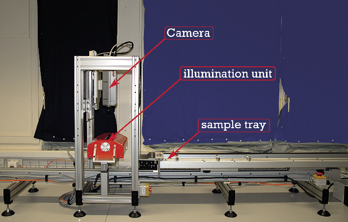
Figure 1: Specim Ltd. hyperspectral core scanner at the Paleolimnology Lab, University of Bern.

Here, we present the first results from the next generation measurement device, a hyperspectral core scanner that combines micro remote-sensing techniques with lake sediment analysis. The Specim Ltd. scanner (Fig. 1) consists of a hyperspectral camera and a sample tray that moves underneath an illumination chamber and the camera slit. The camera takes reflectance spectra from the sediment surface in the range 400–1000 nm with a spectral resolution of 0.8 nm and a spatial resolution (pixel size) as small as 38 x 38 µm. One meter of sediment core is measured in ca. 15 min and produces ca. 45 GB of data. Data normalization and analysis is made using remote sensing software.

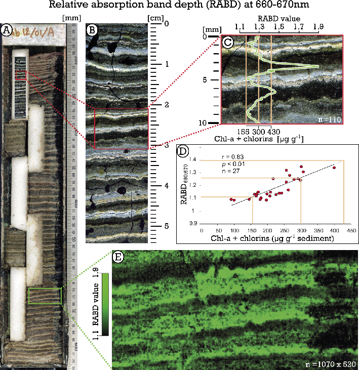
Figure 2: Example of hyperspectral imaging of varves from Lake Żabińskie in Poland. (A) Near-infrared composite image of a sediment core; (B) close-up of a thin section under cross-polarized light; (C) hyperspectral RABD660;670 time series along a cross section of two varves of wet sediment (green line, mean value of 29 pixels width); (D) calibration of spectral imaging data with HPLC data for chl-a and chlorins; (E) map of the hyperspectral RABD660;670 index across three annual varves (light green color indicates high chlorin concentration). The orange lines in (C) and (D) mark the range for which the calibration is valid.

Figure 2 presents the first example of hyperspectral imaging using biochemical varves from Lake Żabińskie, a dimictic lake in the Masurian Lakeland, Poland. The varves are 3-4 mm thick and consist of a white calcite layer formed in early summer and a dark layer composed mostly of aquatic organic matter deposited from late summer until winter.

Figure 2c shows a high resolution RABD660;670 profile covering a two year period. Each varve is represented by 40-60 data points depending on varve thickness. These data can be obtained from fresh sediment cores or from resin embedded polished sediment slabs. The measurements show low chlorin concentrations in calcite layers and high concentrations in dark organic layers. It remains to be tested whether the precise position of the RABD660;670 peak actually represents the timing of the algal bloom in the summer season.

Figure 2d shows the regression between high-performance liquid chromatography (HPLC) measurements of photopigments in dry sediment (after pigment extraction) and RABD660;670 measured on the wet sediment. This suggests that the spectral index used here represents chl-a and chlorins, and that it can be converted into concentration values (µg g-1).

Figure 2e shows the same spectral index but now as a map of RABD660;670 values with 1070 x 520 pixels (individual data points). The optically lighter calcite layers have low chlorin values and appear as darker areas while the green areas reflect the high chlorin concentrations found in the organic-rich layers.

Outlook

The example presented here demonstrates the rich potential of hyperspectral imaging as a relatively novel non-destructive sediment analysis. Further opportunities and challenges are found in the following areas:

• Higher spectral resolution (0.8 nm) potentially allows the detection and diagnosis of further substances and a more detailed speciation (e.g. separation of chl-a from chlorins);

• Very high spatial resolution (pixel size 38 µm) allows sub-varve scale investigation (e.g. seasonality of chl-a production) and the detection of sand-size grains (e.g. macro charcoal and fire history).

• The similar resolution as attained with µXRF scanning allows one to compare these two data types at very high resolution.

• Attributing the spectral properties of sediments to specific substances and minerals (proxy-proxy calibration) remains a great challenge since most of the pixels contain information from a mix of substances. Statistical techniques applied in remote sensing, such as pixel classification, end-member spectra, spectral unmixing, might help to improve the calibration between hyperspectral index data and the concentration of specific substances in sediments. Making this step is fundamental for improving the interpretation of hyperspectral data.

In summary, hyperspectral imaging offers great opportunities for the analysis of lake sediments at the sub-varve scale. The method can also be applied to marine sediments, tree rings or speleothems.

affiliations

1Oeschger Centre for Climate Change Research & Institute of Geography, University of Bern, Switzerland

2GeoConsult Rein, Oppenheim, Germany

3Institute of Geography, University of Gdańsk, Poland

contact

Martin Grosjean: martin.grosjeanoeschger.unibe.ch

references

Das B et al. (2005) Can J Fish Aquat Sci 62: 1067-1078

De Jong R et al. (2013) Clim Past 9: 1921-1932

Debret M et al. (2011) Earth Sci Rev 109: 1-19

von Gunten L et al. (2009) Holocene 19(6): 1-9

Rein B, Sirocko F (2002) Int J Earth Sci 91: 950-954

Takeshi Nakagawa1 and Suigetsu 2006 Project Members2

High-precision depth control is an absolute necessity for varve studies. The Lake Suigetsu 2006 project developed simple yet effective solutions to the most common problems related to core preparation and archival.

Depth control is crucial for all sediment studies and very small differences, even at the mm-scale, can be critical when studying past environmental changes at high resolution. However, achieving and maintaining such precision along a long core is challenging.

Splitting a cylindrical core into sampling and archival halves is common practice, and at some point, when the sediment of the sampling half is already exploited, researchers may wish to take complementary samples from the archive half. But even the seemingly simple task of taking a sample from exactly the same position as in the sampling half is not always easy because cores can expand or contract during storage. Also, tops and bottoms of core sections do not always retain clean and flat surfaces from which precise distances can be measured.

The earlier phase of the Lake Suigetsu project (SG93) revealed such problems; however, most were resolved through innovative techniques developed during the follow-up project that started in 2006 (SG06). This article outlines how we achieved depth control with millimeter or even sub-millimeter precision on a >40 m long quasi-continuously laminated sediment core.

Sampling techniques

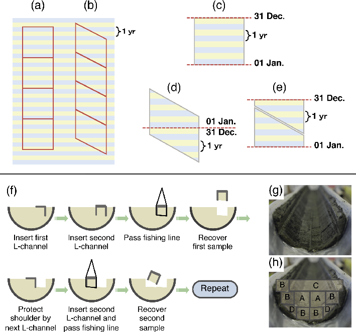
Figure 1: Top. Parallel samples (a) may contain four blue and three yellow “seasonal” layers, or vice versa, depending on sampling position, making the resulting samples incoherent. This effect is considerably reduced in diagonal samples (b). If one could cut samples precisely between 1 January and 31 December, then we would not have the “last seasonal layer” problem (c). Such ideal cutting is not possible in the real world. However, diagonal cutting is almost equivalent to such ideal cutting. Theoretically (i.e. not in practice), it is possible to cut a diagonal sample into two blocks precisely at the transition from one year to the next (d). By flipping the upper and lower blocks of (d), we can obtain a sub-sample (e), which is very close to the ideal cutting (c) in terms of the number of included seasonal layers. Bottom: (f) Procedure to recover multiple LL-channel samples (modified after Nakagawa et al. 2012) and (g-h) an example of intense sub-sampling by double-L (LL) channels. A and B: 15x15 and 12x12 mm LL-channel samples. C: Slab samples for soft X-radiography. D: 12 mm single L-channel samples. 84% of the entire core and 94% of the undisturbed part (i.e. excluding the outer 2 mm) of the core were recovered.

It is common practice to slice varved sediments into regular thin (typically 0.5 or 1.0 cm) disks to avoid depth uncertainties between sub-samples from the same slice. However, this is not ideal because the varved sediment samples are then likely to either under- or over-represent a specific season (Fig. 1a). This is particularly a problem when producing measurements of signals with strong seasonality, i.e. most paleoclimatological proxies. If a sample represents around ten years, such as those typically used for pollen or diatom analysis, inclusion or exclusion of one seasonal layer can result in up to 10% difference in the proxy signal. Indeed, it is mainly for this reason that the pollen data from the precursor SG93 project (e.g. Nakagawa et al. 2003) had a low signal to noise ratio. A simple solution to overcome this problem of introducing a seasonal bias from arbitrarily sampling the 'last seasonal layer' is diagonal cutting. If one can avoid cutting cores into disks, but instead cut them into longitudinal bars and slice these bars diagonally into individual samples, then the “last seasonal layer” of each sample becomes blended (Fig. 1b). Or, in other words, the number of years represented in each sample becomes almost uniform for all seasons. This can be geometrically understood by flipping upper and lower parts of the same sample (Fig. 1c-e).

U-channel sampling is common, especially for paleo-magnetism studies, as a method to obtain longitudinal sediment bars from cylindrical cores. However, it is not easy to take multiple U-channel samples from the same core because the first U-channel makes an exposed fragile “shoulder”, which is very likely to be destroyed by subsequent insertion of a new U-channel. Therefore, for the SG06 project, we invented a double-L (LL) channel (Nakagawa et al. 2012). The LL-channel is almost identical to the U-channel, but consists of two L-shaped angles, which together form the “U” shape. The first L-channel protects the fragile shoulder regions. The second L-channel can then be inserted to produce the combined U-channel. Finally, the sediment underneath is cut with a fishing line to recover the sediment bar from the rest of the core. The LL-channel method allows multiple sampling of the same core section (Fig. 1f), typically allowing >90% of the undisturbed part (i.e. excluding the outer 2 mm) of the core to be recovered (Fig. 1g-h).

Another advantage of the LL-channel technique is that we can remove one of the L-channels after recovering the sample and leave the sediment sitting on only one L-channel. This exposes two sides of the longitudinal sediment bar, instead of just one, as with the U-channel. The exposure of two sides allows an easy diagonal slicing of the bar-shaped samples. This approach is much tidier than digging holes from U-channel samples and provides an almost ideal solution to the problem of the "last seasonal layer". Finally, L-shaped angles are less expensive than specifically manufactured U-channels and are easy to obtain in a range of sizes from hardware stores.

We have also developed relatively simple tools (SG06 Centi-slicer and Milli-slicer) to facilitate the diagonal slicing of LL-channel-derived samples at a regular interval of either 1 cm or 1 mm, respectively. The relevant explanatory video-clips and comprehensive description of sampling techniques can be viewed online.

Precise depth control

Because laminae are not always perfectly parallel and the samples often expand or contract depending on storage conditions, the multiple LL-channel samples do not provide perfectly identical replicates. The distance between a given pair of layers varies across multiple LL-samples from the same section. Slicing those bars at an even interval would not yield sub-samples that are stratigraphically identical. We therefore used an interpolation technique to control depth determinations at sub-millimeter precision.

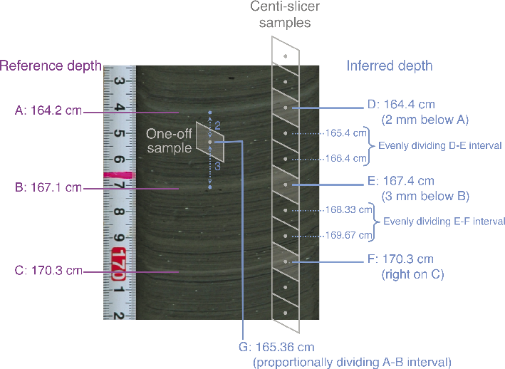
Figure 2: (A-C) Marker layers with reference depth. (D-G) Depths measured relative to the marker layer. The sediment picture is artificially distorted for demonstration purposes in order to enhance the impact of non-horizontal layers.

Alan E.S. Kemp

Laminated marine sediments have the potential for seasonal resolution that can be exploited using scanning electron microscope techniques. This article provides examples of the power of such an approach.

Marine varved and laminated sediments are widely distributed (Kemp 2003). They are not restricted to oxygen-depleted marginal basins with shallow sill depths or to productive shelves and slopes, but are increasingly being found in the deep sea where massive particle flux has suppressed benthic activity, preserving seasonal flux events as sedimentary laminae (Kemp et al. 2006). Scanning Electron Microscope (SEM) methods using back-scattered electron imagery (BSEI) have enabled the identification and sub-sampling of near-monospecific diatom laminae from seasonal blooms and flux events. BSEI, when combined with ecological insights, allows the development of a species-based seasonal approach for climate reconstruction in the marine realm. Highlighted here are new methodologies that have increased the resolution of stable isotope proxy applications to a seasonal scale, and also other integrative studies that have provided insights into interannual climate variability and to the biogeochemical carbon cycle.

Diatom stable isotope records

Figure 1: (A) Back-scattered electron imagery (BSEI) photomosaic of a polished thin section (PTS) of resin-embedded seasonally laminated sediments of deglacial age from Palmer Deep, West Antarctic Peninsula. The core interval shows three seasonal flux laminae: (i) spring diatom lamina dominated by Hyalochaete Chaetoceros spp. resting spores (CRS); (ii) summer terrigenous lamina; and (iii) late summer lamina characterized by high abundances of Thalassiosira antarctica resting spores. (B) BSEI of PTS and (C) topographic SEM images of T. antarctica resting spore lamina (iii). (D) BSEI and (E) topographic SEM images of CRS lamina (i). (F) Seasonal offset between δ18Odiatom for CRS (spring) and T. antarctica RS (summer) sampled from the same year (modified from Maddison 2006 and Swann et al. 2013).

Quantitative paleoceanographic reconstructions of temperature, salinity and ice volume from marine sediments have traditionally used oxygen and carbon isotope analysis of calcite foraminifera shells. However, the resolution of such records is typically centennial at best due to low sedimention rates or low foraminifera abundance in rapidly accumulating sediments. To overcome this limitation and increase the resolution of paleoceanographic research, isotope records are derived from the frustules of diatoms (De La Rocha 2006; Swann and Leng 2009). Near-monospecific diatom blooms can form laminas from millimeters to centimeters in thickness (Fig. 1). The challenge has been to avoid seasonality, habitat, and inter-species effects by isolating diatom samples from a single taxon that grows in a known season and, typically, at known depths in the water column.

The potential for such seasonal-scale isotope proxy resolution is shown by new analyses of sediments from the West Antarctic Peninsula (Swann et al. 2013). In this pioneering study, a micro-manipulator technique has been developed that permits the separation of diatom species for oxygen isotope analysis (Snelling et al. 2013). Two separate species groups were identified as dominant in the laminae: (i) the near-monospecific Hyalochaete Chaetoceros spp. resting spores (CRS) represent spring deposition linked to sea-ice melt; and (ii) the Thalassiosira antarctica resting spores relate to summer deposition. Oxygen isotope analysis of these two species groups, together with coarse and fine diatom fractions from the same samples, have been used to develop records of changes in magnitude of spring melting and changes in the relative importance of spring sea-ice versus summer glacial-ice melting (Fig. 1). These results offer insights into glacial dynamics and ocean-atmosphere variability on seasonally resolved timescales and, more broadly, point to a future treasure trove of archives for quantitative seasonal palaeoclimatic information.

Permanent El Niño hypothesis

Figure 2: (A) Back-scattered electron imagery (BSEI) of seasonally laminated sediments of Cretaceous age from the Alpha Ridge of the Arctic Ocean. (B) Topographic SEM image of spring Chaetoceros-type resting spore lamina. (C) Multi-taper method (MTM) power spectra of time series of resting spore lamina thickness from a 507-year interval showing peaks significant at 99% confidence level in the quasi-biennial and typical ENSO low frequency band (4.1 years). (D) and (E) Wavelet power spectra (D) of the Niño3 SST index from 1871 to 1998 (Torrence and Compo 1998) resampled to annual resolution to mimic laminated data, and (E) a 507-year Alpha Ridge record from the late Cretaceous. Late Cretaceous periodicities in the ENSO-band (broadly, 2-8 years) are non-stationary, that is to say, the dominant frequencies vary with time, and show a striking resemblance to similar behavior in the modern ENSO time series. (Adapted from Figs 2-4 of Davies et al. 2011).

It has been suggested that the present climate may be approaching a threshold or tipping point that may move the Pacific equatorial ocean-atmosphere system into a permanent El Niño state, with far-reaching implications for global climate (Fedorov and Philander 2000; Fedorov et al. 2006). Supporting evidence has come from foraminiferal paleotemperature studies at multi-millennial resolution suggesting that such a permanent El Niño state existed during the Pliocene warm period (Wara et al. 2005). However, new records from laminated sediments and other seasonally resolved archives from ancient greenhouse periods contradict this hypothesis. Corals from the Pliocene (Watanabe et al. 2011), bivalves from the Eocene (Ivany et al. 2011), annual lamina thicknesses from late Miocene evaporites (Galeotti et al. 2010) and Eocene oil shales (Huber and Caballero 2003; Lenz et al. 2010) have all produced robust El Niño signals during warm periods. The application of BSEI to identify sub-annual lamina components has also contributed to this debate. Further evidence comes from the Cretaceous greenhouse period from California, where time series of alternating seasonal diatom and terrigenous sediment laminae record a strong influence of the El Niño–Southern Oscillation (ENSO) on marine productivity, terrestrial rainfall and run-off (Davies et al. 2012). Exceptionally-preserved Cretaceous-age laminated diatomites from the Arctic Ocean that reveal alternating laminae of spring diatom resting spores and late summer and fall vegetative cells (Davies et al. 2009) have been analyzed to produce a thousand-year time series (Davies et al. 2011). Strong cycles in both the quasi-biennial and the 4-5 year ENSO low frequency band indicate robust El Niño teleconnections to high latitude climate, as occurs today (Fig. 2). This extensive, and increasing, evidence from laminated sediments and other seasonally-resolved archives for a continuously dynamic ENSO even during warm periods does not support the permanent El Niño hypothesis.

Marine biological carbon pump

One of the long-standing priorities in oceanographic research is to better understand the workings of the biological carbon pump that draws down CO2 from the atmosphere and exports it to the ocean depths. A widespread view has been that increased warming-induced stratification of the oceans will lead to a shift from diatom production to smaller phytoplankton, reducing the effectiveness of the biological pump and acting as a positive feedback that promotes the build up of atmospheric CO2 concentrations and warming of the atmosphere (Steinacher et al. 2010). However, our current understanding of the biological carbon pump is poor. Many of the algal production events that dominate carbon export are spatially and temporally highly restricted, and subsurface processes are not well captured by the conventional oceanographic observations that are biased towards the surface, typically the topmost ~20 m (McGillicuddy et al. 2007; Lomas et al. 2009). Sediment traps have been used to record flux from the surface ocean but their positions are localized and they only represent, on aggregate, a record of a few centuries. In contrast, over the past ~20 years studies of laminated marine sediments have generated many thousands of years of seasonally resolved time series of sediment deposition in widely distributed locations, covering periods from the Cretaceous to the Holocene.

There has recently been a convergence between new oceanographic observations of diatoms in stratified seas and studies of the same taxa in laminated deep-sea sediments. These show that key large-diatom species may bloom and concentrate in stratified surface waters and generate massive carbon flux exceeding that of the spring bloom. Thus, in opposition to the previously favored ideas, stratified oceans may actually enhance carbon export, drawing down CO2 and providing negative feedback to global warming (Kemp and Villareal 2013).

affiliation

National Oceanography Centre, University of Southampton, UK

contact

Alan E.S. Kemp: aesknoc.soton.ac.uk

references

Davies A et al. (2011) Geophys Res Lett 38, doi: 03710.01029/02010GL046151

Kemp AES (2003) Phil Trans Roy Soc Math Phys Eng Sci 361: 1851-1870

Kemp AES, Villareal TA (2013) Prog Oceanogr 119: 4-23

Snelling AM et al. (2013) Silicon 5: 13-17

Swann GEA et al. (2013) Earth Planet Sci Lett 364: 12-23

Scott St. George

The width of an annual tree ring is without question a very simple indicator of the character of that year’s weather, but collectively, the global network of tree-ring width measurements represents an invaluable resource for high-resolution paleoclimatology.

For over five centuries, it’s been known that the annual growth rings of trees in temperate and boreal forests are shaped by variations in weather and climate (Stallings 1937). It was not until the 1960s, however, that research showed how the environmental information recorded in tree-ring widths can be obscured or sharpened by interactions between climate and ecology (Fritts et al. 1965).

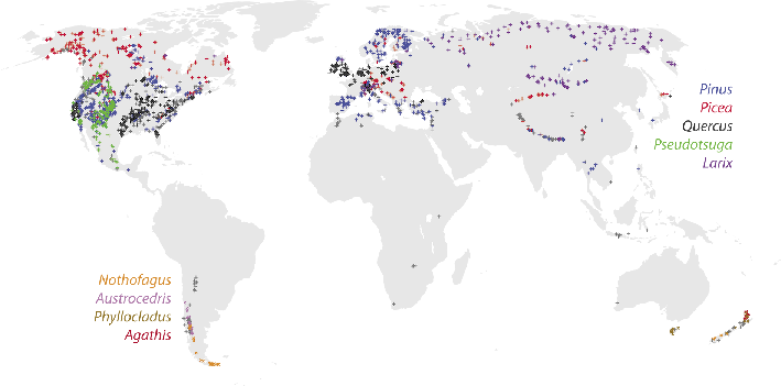
Based on these insights, which established the theoretical foundation for the nascent field of dendroclimatology (Fritts 1976; Cook and Kairiukstis 1990), scientists have spent the last five decades developing tree-ring width records at thousands of locations around the world. In part because these data are so widespread and so massively replicated, the combined network of tree-ring widths is now one of the most important sources of proxy climate information on the planet (Solomon et al. 2007; Mann et al. 2008; Villalba et al. 2012; PAGES 2K Consortium, 2013).

Figure 1: The global network of tree-ring width data held by the World Data Center for Paleoclimatology, NOAA (status 6 July 2012). Colored crosses mark the location of ring-width records from the tree genera most commonly used. Records derived from genera other than those included in the legend are indicated by grey crosses.

The largest archive of tree-ring width data is held within the International Tree-Ring Databank (ITRDB; Grissino-Mayer and Fritts 1997), an open-access database currently maintained by the National Oceanic and Atmospheric Administration (NOAA) in Colorado, USA. Established in 1974 as a permanent repository for digital tree-ring measurements, the ITRDB includes more than 3,200 ring-width records from all continents except Antarctica (Fig. 1). Most records housed by the ITRDB are from North America and Europe, but the archive also includes major regional collections from Siberia (Schweingruber and Briffa 1996), Mongolia (Pederson et al. 2001; Davi et al. 2013), the Tibetan Plateau (Cook et al. 2003; Borgaonkar 2011), the southern Andes (Villalba et al. 2010, 2012), North Africa (Touchan et al. 2011), and New Zealand (Dunwiddie 1979; Ogden and Ahmed 1989). Many more ring-width records are held outside the ITRDB in separate databases operated by research groups and individual scientists.

Recent collection efforts have filled major gaps in the global network in Southeast Asia and India (Cook et al. 2010; Linderholm et al. 2013; Pumijumnong 2013), but despite these successes ring-width records are largely absent from the tropics and much of the Southern Hemisphere. This is either because the climate of these areas is not seasonal enough to induce dormancy in trees (e.g. in areas such as Amazonia, tropical Africa and Indonesia) or is too arid to support forests (e.g. Saharan Africa, the Middle East and central Australia).

Strengths of network-based analyses

Because it is made up of thousands of records, which themselves are built from hundreds of thousands of tree-ring series, the data in the global tree-ring width network are replicated to an extent unequalled by any other high-resolution climate proxy.

For each individual record, ring-width measurements from two to several hundred tree-ring specimens are combined to produce a mean-value function, often called a “chronology”. This averaging procedure amplifies the environmental signals shared by most trees and reduces noise related to non-climatic factors such as tree age or ecological disturbance (Cook 1987; Cook and Pederson 2011).

In the same way, but on a grander scale, large networks of tree-ring records allow the opportunity to assign more weight to behavior shared among many records and tree species, reduce emphasis given to unusual records that may be dominated by non-climatic factors, and (potentially) improve the accuracy of large-scale climate reconstructions (Meko et al. 1993). Networks also allow for the use of reconstruction methods, such as canonical-correlation analysis (Fritts et al. 1971) and principal-component regression (Cook et al. 2004; 2010), that cannot be applied to small sets of ring-width records.

Large networks can also be used to verify relationships between tree growth and climate that have been identified previously within single records or small collections. Some reconstruction approaches, either explicitly or implicitly, conduct an initial screening to select tree-ring records as potential predictors; however, under some circumstances this process can cause records to be incorrectly identified as sensitive to the target climate parameter (Bürger 2007). Statistical experiments conducted on networks of ring-width records can help distinguish between climate-tree relations that are reliable and those that might be artifacts caused by chance (St. George and Ault 2011).

Paleoclimate products based on tree-ring width networks

For several decades tree-ring widths have been one of the main proxies used in high-resolution paleoclimatology (Bradley 2011; Hughes 2011) and these data continue to be used regularly as the sole or leading source for paleoclimate reconstructions spanning the late Holocene.

Figure 2: Drought severity in North America (Cook et al. 2004) and monsoon Asia (Cook et al. 2010) during the late Victorian Great Drought of 1876 to 1878 AD. Cook et al. have used ring-widths and other tree-ring parameters to produce year-by-year maps of summer drought severity (as represented by the Palmer Drought Severity Index) extending back to 1 BC in North America and 1300 AD in Asia.

Many products have exploited the extensive replication and broad distribution of tree-ring networks to develop spatially-explicit estimates of past climate at regional, hemispheric or global scales. The leading example of this approach is provided by the North American Drought Atlas (Cook and Krusic 2004; Cook et al. 1999, 2004, 2007), which used a very large set of moisture-sensitive tree-ring width records to generate yearly maps of drought severity across the continent. A parallel product for monsoon Asia was released in 2010 (Cook et al. 2010) and although these reconstructions also incorporated other tree-ring measurements including sub-annual increments and maximum wood density, tree-ring widths were still the main predictors of past drought (Fig. 2).

Large sets of ring-width data have also provided the foundation for proxy estimates of hemispheric and global surface temperatures (Mann et al. 2008), the first near-continental scale reconstructions of precipitation and temperature in the Southern Hemisphere (Neukom et al. 2010, 2011), and most of the regional reconstructions in the recent PAGES 2k synthesis (PAGES 2k Consortium 2013).

Finally, ring-width networks have been used recently to gauge the relative influence of environmental stressors on forest health (Williams et al. 2012), set real-world targets for process models that simulate tree-ring formation (Tolwinski-Ward et al. 2011; Breitenmoser et al. 2013), and to argue against the hypothesis that major volcanic eruptions caused widespread shutdowns in wood formation in forests across the Northern Hemisphere (St. George et al. 2013; D’Arrigo et al. 2013).

Conclusions

The width of an annual growth ring is without question a very simple indication of a tree’s biological activity and the character of that year’s weather. In spite of that simplicity, the millions of observations that make up the global tree-ring network collectively provide us with a powerful and flexible tool to study forest vigor and climate over a broad range of spatial and temporal scales (Cook and Pederson 2011).

As we develop more and more records that describe tree-ring parameters such as maximum latewood density (Briffa et al. 2004), isotopic composition (Csank 2009) or sub-annual increments (Griffin et al. 2011), it should be possible to use analytical methods first applied to tree-ring widths to improve our understanding of tree-climate relations and identify robust climate signals within these other metrics.

Tree rings offer several advantages as a proxy, including their annual or sub-annual resolution and unmatched dating accuracy. However, beyond the archive’s own intrinsic qualities, the central role played by ring-width records in modern paleoclimatology is also due to the global network’s massive replication and widespread geographic coverage. Those qualities are testament to the dendrochronological community’s long-standing commitment to field collection, record development, and data sharing.

acknowledgements

I am grateful to Bruce Bauer (NOAA), David Meko (University of Arizona), and Toby Ault (Cornell University) for sharing meta-data and code needed to produce the global map of tree-ring widths.

affiliation

Department of Geography, Environment and Society, University of Minnesota, USA

contact

Scott St. George: stgeorgeumn.edu

selected references

Full reference list under: pastglobalchanges.org/products/newsletters/ref2014_1.pdf

Cook ER et al. (2010) Science 328: 486-489

Fritts HC (1976) Tree Rings and Climate, Academic Press, 582 pp

Grissino-Mayer HD, Fritts HC (1997) The Holocene 7: 235-228

Neukom R et al. (2010) Geophysical Research Letters 37, doi: 10.1029/2010GL043680

Williams AP et al. (2012) Nature Climate Change 3: 292-297

Chris Turney1, J. Palmer1, K. Allen2, P. Baker2 and P. Grierson3

To overcome the relative dearth of paleoclimate records in Southern Hemisphere mid-latitudes, new methods are being developed in Australasia to exploit the potential of tree rings across the region.

Figure 1: Location of Australasian tree-ring sites discussed in the text with major climatic and oceanographic boundaries shown. ITCZ denotes Intertropical Convergence Zone, LC the Leeuwin Current, EAC the East Australian Current, TF the Tasman Front, STF the Sub Tropical Front, and SAF the Subantarctic Front.

The Australasian region is potentially highly sensitive to climate change, including abrupt transitions caused by the crossing of thresholds within different components of the climate system (Fig. 1). Accurate reconstructions of the past behavior of the climate system are needed to better understand the mechanisms, and to validate projections of future change at the junction between tropical and polar regions (PAGES 2k Consortium 2013). Tree-rings are critical in this regard.

Over the 20th century, dendroclimatic research in the Northern Hemisphere has advanced in leaps and bounds. In the Southern Hemisphere the much smaller land mass and less amenable tree species have limited the development of long proxy climate records from trees. However, during the past five years, significant technical advances and discoveries have created an exciting set of opportunities for increasing the quality and understanding of tree-ring-based climate reconstructions in the Australasian region and, potentially, other tree-bearing regions of the world.

Tree ring growth analysis

Like most proxy-climate reconstructions, those from tree rings are developed from statistical models relating observed climate data to measured tree-specific features such as ring widths. While these models are typically based on the correlation between two variables, causation is inferred from detailed understanding of the physiological mechanisms that drive tree growth and tree-ring formation. Recent technological and analytical advances have created the potential to monitor radial growth and wood cell formation at sub–hourly resolution over multiple years (Drew and Downes 2009). For the first time, this enables an assessment of the role of weather and climate in tree–ring formation for long-lived trees of global paleoclimatic importance from Australia and New Zealand (Drew et al. 2013; Wunder et al. 2013).

Wood properties beyond ring-width

Particular interest has been focused on the recent development of tree-ring chronologies based on wood microfibril angle (MFA; angle of cellulose microfibrils in the cell wall relative to the long axis of the cell) and tracheid radial diameter (TRD). Both exhibit a strong temperature sensitivity during the austral summer, i.e. November to April (Drew et al. 2013), extending across much of temperate south-eastern Australia (Allen et al. 2013). This development is particularly important as the wood-property chronologies were developed from samples that exhibited no sign of a climate signal in ring width, although the wood-properties based results appear stronger and more temporally stable than the widely cited Mt Read summer temperature reconstruction from Tasmanian Huon pine (Cook et al. 2000). As these authors point out, the results demonstrate the potential of wood property chronologies to open up vast areas for dendroclimatic research in data-sparse regions of Australasia, and beyond, where standard ring-width chronologies have provided little dendroclimatic value.

Investigating divergence

The relative paucity of climate-sensitive, multi-millennial tree-ring chronologies in the Southern Hemisphere makes it particularly important to examine whether the existing chronologies exhibit signs of anomalous growth reduction (the so-called ”divergence problem”), as identified in the Northern Hemisphere (D’Arrigo et al. 2008). A program is currently underway to update long, climate-sensitive chronologies in the Southern Hemisphere as many lack ring-width data from the last 20 years or more. The investigation includes an assessment of several factors: the impact of various methods of standardization; the impact of signal-free processing (Melvin and Briffa 2008); and whether or not relationships between climate and wood-properties (e.g. density, TRD, MFA) may be more temporally stable than for ring-width. In addition, high-resolution data will provide a better empirical understanding of the climate response of trees at key sites (Fig. 1) and of the mechanisms underpinning any observed patterns of divergence between tree-ring properties and climate.

Filling in knowledge gaps

The eucalypts and acacias that dominate the Australian landscape generally lack discernible annual growth rings and, until recently, have not been considered suitable for climatic reconstructions (Brookhouse 2006). However, annually-resolved tree-ring chronologies have been recently developed from selected high-elevation species of these genera. The early despondent reports of the poor potential for tree-ring chronologies across much of Australia is being overcome by the development of a range of new chronologies that are based on measurements of ring width coupled with δ13C and δ18O isotope data. To date, these studies have mostly focused on long-lived Callitris trees that occur across much of inland Australia (Baker et al. 2008; Cullen and Grierson 2009). Other notable advances include using the methodological approach of “reverse-latewood”, which is characterized by a sharp transition from earlywood- to latewood-type fiber tracheids followed by a gradual transition from latewood into earlywood (Brookhouse et al. 2008); chronology development from the only Australian alpine conifer (McDougall et al. 2012); and preliminary climate reconstructions based on the sub-tropical Toona ciliata (Heinrich et al. 2008). Finally, new techniques using 14C-wiggle-matching have further enhanced the capacity to accurately date tree-ring chronologies in Australasia (e.g. Wood et al. 2010).

When these techniques are coupled with isotope analysis, wood density and elemental chemistry it should be possible to identify common sequences or patterns in reconstructions that reflect regional hydroclimatic histories (Evans et al. 2013), including the frequency of cyclones that drive rainfall patterns across much of northern Australia (Cullen and Grierson 2007). Such an approach is needed to provide the spatial infilling crucial for exploring teleconnections and their temporal stability, particularly regarding the influence of climate modes, such as the El Niño-Southern Oscillation, the Southern Annular Mode and the Indian Ocean Dipole, on the Australasian region (e.g. Neukom and Gergis 2010).

Reconstructing changes in the carbon cycle

Figure 2: Ancient kauri tree (Agathis australis) prior to commercial processing in Northland, New Zealand (Jonathan Palmer pictured for scale).

Despite considerable effort, the reliable tree-ring dated section of the most recent internationally-accepted calibration curve (IntCal13; Reimer et al. 2013) based on North American and European trees extends back only to 12.59 cal ka BP (Schaub et al. 2008). An exciting Southern Hemisphere possibility for radiocarbon calibration exists in the form of subfossil kauri trees buried in bogs scattered over a 300 km stretch of northern New Zealand (Palmer et al. 2006). We know of nowhere else in the world with such a rich resource of subfossil wood that is capable of capturing the complete temporal range of radiocarbon. The time span preserved within these bogs covers more than 130 ka. These trees are of vast proportions and almost perfectly preserved (Fig. 2); individual trees can measure up to 4 m across and live for up to 2000 years. Within this precious archive is an annual record of past climate but, equally importantly, of changing atmospheric radiocarbon levels. The kauri trees have considerable potential to assist in the development of a Southern Hemisphere component of a unified global calibration curve. In addition, the tree-ring sequences can be superposed on other radiocarbon records to constrain carbon cycling in marine and atmospheric reservoirs at times of abrupt change (Turney et al. 2010). Most recently, the detailed analysis of kauri trees has been used to identify errors in Northern Hemisphere radiocarbon datasets (Hogg et al. 2013), providing a more accurate calibration for the transition to the Holocene, and potentially for the last glacial period.

affiliations

1Climate Change Research Centre, University of New South Wales, Kensington, Australia

2Melbourne School of Land and Environment, University of Melbourne, Richmond, Australia

3School of Plant Biology, The University of Western Australia, Crawley, Australia

contact

Chris Turney: c.turneyunsw.edu.au

references

Allen K et al. (2012) Dendrochronologia 30: 167-177

Baker P et al. (2008) Aust J Bot 56(4): 311-320

Cullen LE, Grierson PF (2009) Clim Dyn 33: 433-444

PAGES 2k Consortium (2013) Nat Geosci 6(5): 339-346

Bernd R. Schöne1 and Donna Surge2

Shells of bivalve mollusks provide time-constrained, multi-proxy records of climate change in any aquatic setting with unprecedented temporal resolution ranging from years to individual days. We explain why this archive is unique and list current research foci.

Climate proxy-data are crucial to better understand natural environmental variability prior to the instrumental era (Jones et al. 2001). In particular, there is a need for more sub-seasonal to annual resolutions of well-constrained and quantifiable proxy data from environmental settings for which only limited data are available, e.g. in coastal marine regions and mid- to high-latitude oceans (Solomon et al. 2007). Sclerochronology describes the investigation of the growth patterns and geochemical properties of the skeletal hard parts of bivalve shells. During the last decade, many sclerochronological studies (e.g. Schöne and Gillikin 2013) have confirmed that bivalve shells can record climate at sub-seasonal time scales (Butler et al. 2013; Schöne et al. 2003; Wanamaker et al. 2012).

Bivalve shells as paleoclimate archives

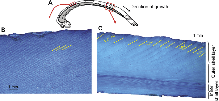
Figure 1: Growth patterns in bivalve shells (example: Arctica islandica). (A) Schematic cross-section showing internal growth patterns in the outer (white) and inner (gray) shell layers. Polished sections stained with Mutvei’s solution show daily (B) and annual (C) growth patterns in the outer shell layer. Growth lines (marked yellow in B and C) delimit growth increments.

Bivalve shells can provide a precise chronology because calcium carbonate is periodically accreted to all growing shell margins (Barker 1964; Clark 1974; Jones 1980; Schöne and Surge 2012; Fig. 1). Regularly changing rates of skeletal formation are controlled and maintained by so-called biological clocks, which are constantly reset by environmental pacemakers (light, tides, food availability, etc.; Kim et al. 2003; Williams and Pilditch 1997). These internal time-keeping mechanisms ensure that the shell growth pattern is divided into time slices of approximately equal duration (Dunca and Mutvei 2001; Witbaard et al. 1997), which produce growth increments and growth lines. Growth increments represent periods of fast growth and growth lines periods of slow growth. Together, they are prerequisite for sclerochronological analyses because they can be used to measure time, and place each shell portion into a precise temporal context. Periodic growth patterns in bivalves include annual cycles (Jones and Quitmyer 1996; Pulteney 1781; Weymouth 1922), fortnightly cycles (15 and 13.5 lunar days; Evans 1972; House and Farrow 1968; Ohno 1989), as well as circadian (ca. 24 hours; Schwartzmann et al. 2011), circalunidian (lunar-daily, ca. 24.8 hours; Richardson 1987), circatidal (semidiurnal, ca. 12.4 hours, ebb/neap tide cycle; Beentjes and Williams 1986) and ultradian cycles (periods of minutes to hours; Rodland et al. 2006). This makes shells unrivaled archives for measuring time in the geological past at high resolution.

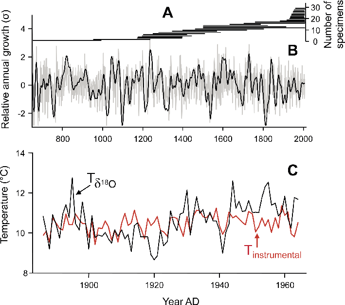
Figure 2: A 1357-year master chronology of Arctica islandica from the North Icelandic shelf (data from Butler et al. 2013). (A) Sample depth. Each horizontal line indicates the lifespan of one specimen. (B) Stacked record of growth increment width-chronologies of the 30 specimens shown in (A). The black line represents the 30-year low-pass filtered annual growth data (gray). (C) Growth increment data can be combined with high-resolution geochemical analysis. The example from Schöne and Fiebig (2009) illustrates the annual temperature evolution in the southern North Sea during the late 19th and the 20th century reconstructed from δ18Oshell values. Instrumental sea surface temperatures are given for comparison.

Bivalve shells also function as faithful and sensitive recorders of environmental change (Fig. 2). Like other cold-blooded animals, bivalve growth is largely controlled by external energy input in the form of temperature, and food quantity and quality. As a result, relative changes in shell growth, expressed through varying increment widths, can provide information on changes in these environmental variables (Kennish and Olsson 1975). Furthermore, the ambient physicochemical conditions (salinity, water quality and temperature, food availability, etc.) that prevailed during its growth are also preserved in the shell as geochemical and crystallographic properties. For example, shell oxygen isotope ratios (δ18Oshell) provide an ideal means to estimate past water temperature and salinity because almost all bivalve species form their shells very close to oxygen isotopic equilibrium with the ambient environment (Epstein et al. 1953; Wefer and Berger 1991).

Whereas the life of some bivalves such as Donax variabilis ends only after a few months (Jones et al. 2005), some species of the class Bivalvia are extremely long-lived (Schöne et al. 2005; Thomson et al. 1980; Zolotarev 1980), and lead the list of the longest-lived solitary (non-colonial) animals. For example, the Pacific geoduck (Panopea generosa) reaches a lifespan of 160 years (Strom et al. 2005), the European freshwater pearl mussel (Margaritifera margaritifera) can live for well over 200 years (Mutvei and Westermark 2001), and lifespans exceeding 500 years have been reported from the deep-sea oyster Neopycnodonte zibrowii (Wisshak et al. 2009) and the ocean quahog, Arctica islandica (Butler et al. 2013). Thus, individual fossil shells open multi-century windows into past climate and provide details on paleoseasonality as well as quasi- and multi-decadal climate variability. However, such analyses are not limited to climatic snapshots. Since contemporaneous specimens from the same habitat exhibit a common response to changing environmental conditions, growth increment width-chronologies of specimens with overlapping lifespans can be combined by wiggle-matching (cross-dating) to form composite chronologies covering centuries to millennia (Butler et al. 2013; Jones et al. 1989; Lohmann and Schöne 2013; Marchitto et al. 2000; Witbaard et al. 1997; Fig. 2). With just one calendar date (e.g. the date of death of live-collected specimens), each sample can be aligned to reveal a complete chronology.

Bivalves exhibit an impressively broad and unrivaled biogeographic distribution. They have adapted to a wide range of different aquatic habitats. Today, bivalves occur in the tropics and near the poles, in shallow waters and in the deep sea, and inhabit the whole range from hypersaline to freshwater settings. Furthermore, bivalves occur abundantly in the fossil record. In fact, their evolutionary history started early in the Cambrian, i.e. 500 Ma ago. Since humans settled along the coasts tens of thousands years ago and exploited shallow marine resources, a vast number of bivalve shells are also preserved in archeological shell middens, i.e. ancient domestic waste deposits. To date, this material has largely been used to infer human subsistence practices by reconstructing the season of collection of the bivalves (Andrus 2011; Burchell et al. 2013).

Current research foci

Growing interest in bivalve sclerochronology over the last decade has fuelled a soaring number of publications and research projects and four main research directions: (1) construction of millennial-scale master chronologies; (2) paleoclimate snapshot analysis (climate reconstruction from single specimens); (3) identification of chemical disequilibrium effects and quantification of vital and possible kinetic effects in order to optimize existing and develop new climate proxies; and (4) season-of-collection studies in archeology and anthropology. Recently, a large collaborative research initiative was funded by the EU (ARAMACC.com), whose goals include: (1) construction of millennial-scale Arctica islandica master chronologies from different settings in the boreal North Atlantic to produce paleoclimate reconstructions using stable isotopes (δ18Oshell, δ13Cshell), Sr/Ca ratios and growth-increment widths; and (2) development of novel bivalve shell-based paleoclimate proxies on the basis of microstructures (overall fabrics, shell architectures), or trace and minor elements. This will require stronger cross-disciplinary collaboration with biochemists to better understand the mechanisms of biomineralization in bivalves, in particular the complex pathways and fractionation processes involved in the transport of elements from the ambient environment to the site of calcified tissue formation (Marin et al. 2012).

The future of bivalve sclerochronology

The potential of bivalve sclerochronology in the fields of archeology and anthropology, evolution, retrospective environmental monitoring, and ecology is still waiting to be fully exploited; however, it will likely have a significant impact on paleoclimate and paleoenvironmental studies. Linking different high-resolution paleoclimate archives advances our knowledge of coupled climate systems, which will further improve predictive numerical climate models. The ubiquitous occurrence of bivalves in shallow-marine settings, especially longer-lived species, makes them suitable candidates for the construction of long master chronologies in both hemispheres. This would, for example, permit deeper analyses of cross-hemispheric climate dynamics in the future.

affiliations

1Institute of Geosciences, University of Mainz, Germany

2Department of Geological Sciences, University of North Carolina, Chapel Hill, USA

contact

Bernd R. Schöne: schoenebuni-mainz.de

selected references

Full reference list under: pastglobalchanges.org/products/newsletters/ref2014_1.pdf

Butler PG et al. (2013) Palaeogeog Palaeoclimatol Palaeoecol 373: 141-151

Jones DS (1980) Paleobiology 6: 331-340

Schöne BR, Gillikin DP (2013) Palaeogeog Palaeoclimatol Palaeoecol 373: 1-5

Schöne BR, Surge DM (2012) In: Selden PA (Ed) Treatise of Invertebrate Paleontology, Part N (Mollusca, Bivalvia), Treatise Online 46, 1-24

Wanamaker AD et al. (2012) Nat Commun 3, doi: 10.1038/ncomms1901

Liangcheng Tan1, I.J. Orland2 and H. Cheng2,3

New analytical techniques enable the extraction of annual climate information from speleothems for times long before historical climate records began.

Speleothems (stalagmites, stalactites and flowstones) are natural paleoclimatic and paleoenvironmental archives. They are widespread in karstic environments and grow from drip water that degases CO2 upon entering caves (Fairchild and Treble 2009). If seasonal climate variations outside the cave (e.g. precipitation, temperature, snow melting) or inside the cave (e.g. humidity, air CO2 partial pressure, air ventilation) are large enough, this seasonality may be preserved as annual laminas in the speleothems (Tan et al. 2006; Baker et al. 2008). Therefore, speleothems have the potential to record past climate with annual resolution.

Annual laminas in speleothems

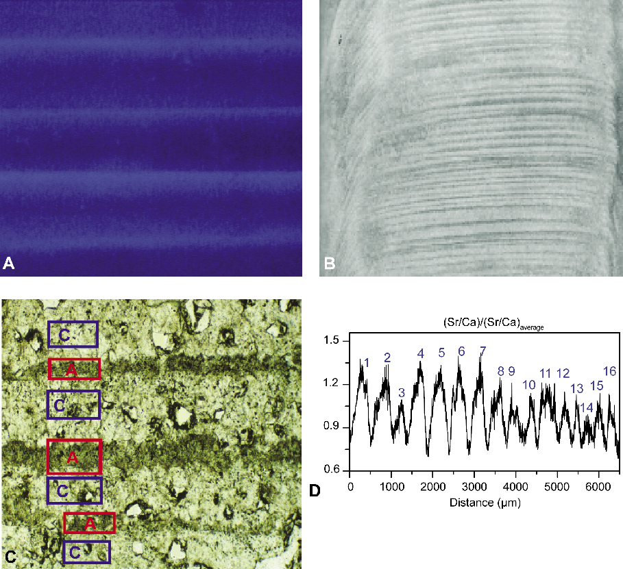
Figure 1: Four types of speleothem laminas. (A) Fluorescent laminas excited by UV light. (B) Visible laminas observed under reflected-light microscopy. (C) Calcite (C) and aragonite (A) couplets, observed under transmitted-light microscopy, and (D) geochemical laminas where the normalized Sr/Ca peaks were used to define 16 years. Modified from Tan et al. (2006) and Johnson et al. (2006).

Four main types of speleothem laminas have been reported (Fig. 1): (1) fluorescent laminas, which can be observed by using conventional mercury light-source UV reflected-light microscopy (Shopov et al. 1994) and confocal laser fluorescent microscopy (Orland et al. 2012); (2) visible laminas, which can be observed using conventional transmitted and reflected-light microscopy (Genty and Quinif 1996); (3) calcite-aragonite couplets, which show seasonal alternations of calcite and aragonite growth layers (Railsback et al. 1994); and (4) geochemical laminas (Johnson et al. 2006) defined by the annual variability of their chemical constituents such as stable isotopes (δ18O, δ13C) and trace elements (e.g. Mg, Sr, Ba). To confirm the annual character of banding, the number of layers counted in a speleothem is compared with the duration of growth measured independently by radiometric dating techniques. For samples of late Pleistocene age, 230Th dating is used most commonly (Baker et al. 1993; Tan et al. 2000), while samples younger than 150 years can be dated with 210Pb and 226Ra methods (Baskaran and Iliffe 1993; Condomines and Rihs 2006) or with the atomic bomb testing 14C signature that characterizes the last 50 years (Genty et al. 1998; Mattey et al. 2008).

Application in paleoclimate studies

The annual laminations in speleothems provide accurate age indications for paleoclimate proxies measured within the speleothem, and allow reconstructing the accurate timing and structure of abrupt climate changes. The temporal relationships between the regional expressions of an abrupt event are crucial for understanding its origination and its transferring mechanisms. For example, Liu et al. (2013) reconstructed the timing and structure of the 8.2 ka event in the East Asian monsoon region based on δ18O and Mg/Ca ratios of a stalagmite from central China. Their results show that the duration and evolution of precipitation during this event is indistinguishable from temperature recorded in Greenland ice cores, suggesting a rapid atmospheric teleconnection between the North Atlantic and the East Asian monsoon region. Likewise, δ18O records from other Chinese stalagmites indicate that the Asian monsoon transition into the Younger Dryas (YD) extended over ca. 340 years (Liu et al. 2008; Ma et al., 2012), while the shift out of the YD took less than 38 years (Ma et al. 2012).

Precise chronologies are also crucial for comparing proxies from speleothems with instrumental meteorological data to identify their climatic and environmental significances. For example, Baker et al. (1998) found a correlation between the content of high-molecular-weight organic acids and annual rainfall in an annually laminated stalagmite from England, and used this correlation to reconstruct precipitation during the last interglacial. In a stalagmite from central Belize, variations of δ13C co-vary with the observed Southern Oscillation Index (Frappier et al. 2002) and were shown to be influenced by changes to the carbon budget of the overlying rainforest. The forest is sensitive to the local weather and, in turn, controlled by the Southern Oscillation.

The layer thickness of annual laminas can be used to infer the speleothem growth-rate per year. Growth rates have been used to quantitatively reconstruct past temperature (Tan et al. 2003), as well as precipitation and associated changes in atmospheric circulation (Proctor et al. 2000).

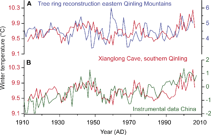
Figure 2: Comparison of temperature from September to May reconstructed by speleothem layer thickness from Xianglong Cave in southern Qinling Mountains, central China (red lines) with (A) tree ring-based winter temperature reconstruction from nearby, and (B) surface winter temperature across China during the last hundred years. Modified from Tan et al. 2013.

Tan et al. (2006) reviewed the applications of stalagmite laminas to paleoclimate reconstructions and compared them to the dendroclimatological approaches. Baker et al. (2007) suggested that a transfer function reflecting the mixing of water from rainfall events and groundwater storage could be used to reconstruct high-resolution hydroclimatic records from stalagmites. More recently, Tan et al. (2013) developed a two-variable linear regression between stalagmite growth rate and temperature that accounts for smoothing and lag effects of stalagmite growth in response to climatic changes. With this regression, they quantitatively reconstructed temperature changes from September to May between AD 1912 and 2006. This stalagmite-based reconstruction is coherent with a nearby tree-ring temperature reconstruction (Fig. 2), which documents the sensitivity of this archive to air temperatures (Tan et al. 2013).

Perspectives

Annually laminated speleothems are often found in caves with a shallow depth and an outside climate that exhibits strong seasonality (Tan et al. 2006). Recent methodological advances have the potential to expand the applications of speleothems as paleoclimate recorders and to reduce their uncertainties in climate reconstruction. For example, digital image analysis, e.g. with a hyperspectral scanner, allows for faster and more accurate counting of laminas compared to traditional optical analyses (Jex et al. 2008). High-precision and high-resolution in situ measurements of stable isotopes and trace elements using ion microprobe (Orland et al. 2009), laser-ablation inductively coupled plasma mass-spectrometry (Johnson et al. 2006), and synchrotron radiation micro X-Ray fluorescence (Borsato et al. 2007) have all revealed annual and sub-annual variations in speleothem chemistry. As a result, improved speleothem chronologies can be built by measuring geochemical variability along the growth axis. Furthermore, by pairing images of annual laminas with seasonal-resolution measurements of geochemical variability in speleothems, seasonal climate patterns can be reconstructed. For example, the combination of fluorescent imaging and ion microprobe analysis of δ18O in speleothems from Israel has been used to identify regional changes in seasonality across abrupt climate events and over millennial time scales (Orland et al. 2009, 2012).

Future research should focus on quantitative and qualitative reconstructions of paleoclimate and paleoenvironment by using multiple proxies from annually laminated speleothems, including stable isotopes, trace elements, as well as layer thickness. Finally, efforts are being made to apply statistical approaches better suited to reconstruct past climate quantitatively using speleothem records (Tan et al. 2006, 2013).

acknowledgements

This study was supported by the Chinese and US NSF, and the Chinese Basic Research Program and Academy of Sciences.

affiliations

1Institute of Earth Environment, State Key Laboratory of Loess and Quaternary Geology, Xi’an, China

2Department of Earth Sciences, University of Minnesota, Minneapolis, USA

3Institute of Global Environmental Change, Xi’an Jiaotong University, Xi’an, China

contact

Liangcheng Tan: tanlchieecas.cn

selected references

Full reference list under: pastglobalchanges.org/products/newsletters/ref2014_1.pdf

Baker A et al. (2008) Int J Speleol 37(3): 193-206

Johnson KR et al. (2006) Earth Planet Sci Lett 244(1): 394-407

Orland IJ et al. (2012) Geochim Cosmochim Acta 89: 240-255

Tan L et al. (2013) Quat Sci Rev 72: 137-145

Tan M et al. (2006) Quat Sci Rev 25: 2103-2117

Ian J. Fairchild1, M. Bar-Matthews2, P. M. Wynn3 and I. J. Orland4

Seasonal signals are transmitted to speleothems via the quantity, chemistry and isotopic composition of dripping water in caves. Modern techniques allow seasonality to be interpreted through variations in trace elements, stable isotopes, and organic fluorescence within annual layers.

Records from calcareous cave deposits (speleothems) can reveal large-scale variations in the climate system over long time periods (Bar-Matthews et al. 2003; Fairchild and Baker 2012). These records require the direct transmission of an atmospheric signal to the speleothem, and uranium-series dating to construct a precise and accurate age model (Cheng et al. 2009). As with other natural archives, ambiguities remain with the climatic interpretation of speleothem records. For example, the mean oxygen isotope composition of speleothems in monsoon-influenced areas has been interpreted as indicating the relative strength of summer versus winter monsoons (Wang et al. 2001). Hence, it is desirable to resolve and understand seasonal processes, particularly those related to rainfall (Johnson et al. 2006; Hu et al. 2008; Orland et al. 2009, 2012). However, how are seasonal signals captured in a cave?

Cave climate and seasonality

Seasonal changes are muted in cave interiors, which are archetypically isothermal, fetid and humid. Therefore, temperatures are usually close to the external annual mean. The difference in external and internal temperatures can lead to density-driven air circulation, which is typically enhanced in the winter, which is also the season of lower levels of CO2 in the cave atmosphere. This leads to more degassing of CO2 from dripwaters and causes speleothems to grow faster in winter than in summer (Wong et al. 2011). A common consequence of this seasonal bias in calcite precipitation is seasonal oscillation of 13C, Mg and Sr concentrations in speleothems (Fairchild et al. 2000; Frisia et al. 2011; Tremaine and Froelich 2013).

The flow-path of dripwater into the cave can also affect the preservation of seasonal signals in speleothems. Overlying karstic carbonate bedrock contains fractures that provide a rapid routing of water away from the surface, while networks of finer pores in the matrix only enable seepage flow. Fracture and pore flow are mixed in varying proportions in dripwaters. Therefore, the quantity and chemical composition of dripwater reflect the magnitude and pattern of rainfall or snowmelt and the pathways of its delivery to the karst system via the overlying soil.

A range of potential consequences arises from the drip-specific hydrological regime – thin laminae in speleothems contain chemical impurities from rainfall infiltration events whereas the dry season usually results in enrichments in trace elements (Baker et al. 2000; Fairchild et al. 2000; Fairchild and Treble 2009). When travel times of water are short, seasonal variations in the oxygen isotope composition of rainfall are transmitted to caves and speleothems, but sites fed purely by seepage flow may have seasonally invariant δ18O compositions. Crucially, these properties can vary between adjacent speleothems in the same cave because of local variations in hydrological properties of the host rock. Hence, for scientists wanting to study climate at high resolution, a cave with speleothems is like the “à la carte” menu to a food-allergy sufferer: careful selection of what item to choose is vital.

Annual and sub-annual properties of speleothems

Figure 1: Three annual growth cycles in a speleothem from the Obir cave, Austrian Alps (Obi84) depicting relative concentrations of lead (Pb), zinc (Zn) and sulfur (S; known to be in the form of sulfate by absorption studies) mapped by micro-XRF synchrotron radiation. High-intensity banding (“greener”) represents transport of organic-ligand-bound Pb and Zn during synoptic rainfall events. Highest intensity bands represent intense autumnal rainfall and loss of organic molecules and associated metals from the soil zone during times of vegetation dieback. Relative concentrations of S demonstrate independent verification of seasonality and timing of the autumnal flush of Zn and Pb. Low winter S concentrations are a product of low cave chamber PCO2 and high carbonate to sulfate ratios during speleothem growth. From Wynn et al. (2014) with permission.

Annual lamination has been established as a common feature of stalagmites under a variety of climatic conditions (Baker et al. 1993; Orland et al. 2009). One type of lamination consists of narrow bands enriched in soil-derived organic matter. These bands are made visible by fluorescence microscopy. The laminae are enriched in trace elements (Borsato et al. 2007), which travel in water and are bound to organic ligands in colloids (Fairchild and Baker 2012). Background transmission of seepage waters containing fine humic molecules with a particular trace element signature should be distinguished from pulses of coarse colloids, which require hydrologically active conditions for their trace element patterns to be recorded (Hartland et al. 2012). Figure 1 illustrates what is perhaps the highest number of precipitation events in a single year ever documented in speleothems (Wynn et al. 2014). In Obir Cave in the Austrian Alps, high levels of lead and zinc, derived from local bedrock, record infiltration from individual synoptic rainfall events. Sensitivity is higher in autumn when vegetation dieback facilitates leaching loss of humic substances and of associated metals from the soil (Borsato et al. 2007).

The time of year is independently documented by the sulfate content of the calcite (analyzed as sulfur; Fig. 1). More sulfate ions are incorporated at high PCO2 (cave air CO2 partial pressure; Frisia et al. 2005). In the Obir cave PCO2 is higher during summer when the external air is warmer (and hence air density is lower) than in the cave. Thus, each summer and winter can be identified as high- (green-colored) and low-sulfate (blue-colored) zones in the speleothem, respectively (Fig. 1). Year-to-year variations in the seasonal sulfate oscillations can reveal the relative length of the warm and cold seasons.

A second type of annual lamination consists of couplets, alternately richer and poorer in fluid inclusions, varying in Mg-Sr chemistry and sometimes differing in mineralogy (Baker et al. 2008). Fundamentally, these laminae reflect an annual bimodality of water chemistry which usually can be correlated with either alternating warm and cold seasons that lead to varying PCO2 levels, or with summer drought, which leads to increases in Mg, Sr and δ13C (Mattey et al. 2008; Boch et al. 2011; Orland et al. 2014).

Figure 2: Examples of four patterns (A-D) of fluorescent banding and δ18O variability observed on annual growth bands in a stalactite from Soreq Cave (Israel) that grew from 34 to 4 ka. A schematic of each pattern is shown above an example from the speleothem. The spots analyzed for δ18O by ion microprobe are marked by red dots, ~10 μm in diameter, on the image of fluorescent banding acquired by confocal laser fluorescent microscopy. Green triangles and blue crosses mark δ18O values measured in areas of bright and dark fluorescence, respectively; each with 2σ error bars. Note the range of δ18O analyses within single bands varies from 0 to >2‰ (Figure adapted from Orland et al. 2012, which includes a climatic interpretation of these patterns).

The changing isotopic composition of water molecules is preserved in the δ18O signal of speleothem CaCO3. The δ18O variation within annual laminae can reflect the seasonal variability in composition of infiltrating water as well as the rainfall amount. However, evaporation in the soil zone and dampening of the seasonal signal by mixing processes during the infiltration can also influence the δ18O values (Ayalon et al. 1998).

A modern well-dated speleothem from Soreq Cave in Israel has revealed characteristic properties that can be used to trace the nature of seasonality and rainfall variability over time. Annual laminae are marked by fluorescent zones that are brighter in wetter years and are associated with δ18O variation. The range of δ18O correlates with the amount of rainfall in the corresponding year (Orland 2012). In older speleothems from Soreq Cave (Fig. 2), changes in the patterns of fluorescent banding and annual δ18O variability are also interpreted to reflect different seasonal climate regimes (Orland et al. 2012).

Analytical frontiers

The identification of sub-annual properties in speleothems depends on the presence of fast-growing, compact crystals (columnar fabrics are best, Frisia et al. 2000) with a growth surface that is either flat, or, if irregular, can be clearly imaged (Fig. 2). For trace elements, the µm-scale resolution of X-ray fluorescence analysis by synchrotron radiation provides the highest resolution that can be obtained to date. SIMS (secondary ionization mass spectrometry) has a resolution of several microns and provides unique data on elements that are difficult to analyze by other means (Fairchild et al. 2001). Accurate and precise laser-ablation inductively coupled plasma mass spectrometry (LA-ICPMS) has ~10 μm resolution, which is sufficient to resolve seasonal properties for faster growing samples. For stable isotopes, faster-growing samples can be sub-sampled by micromilling with a resolution of ~100 μm and analyzed by mass spectrometry (Drysdale et al. 2012). Laser ablation offers a more rapid alternative for stable isotope analysis if care is taken to screen out artifacts (Spötl and Mattey 2006). The oxygen isotope SIMS analysis of Figure 2 was achieved with a spot size of 10 μm, resolving seasonal variations in bands as narrow as 20-30 μm (Orland et al. 2009, 2012).

affiliations

1School of Geography, Earth and Environmental Sciences, University of Birmingham, UK

2Geological Survey of Israel, Jerusalem, Israel

3Lancaster Environment Centre, Lancaster University, UK

4Department of Earth Sciences, University of Minnesota, Minneapolis, USA

contact

Ian J. Fairchild: i.j.fairchildbham.ac.uk

selected references

Full reference list under: pastglobalchanges.org/products/newsletters/ref2014_1.pdf

Fairchild IJ, Baker A (2012) Speleothem Science. From Process to Past Environments. Wiley-Blackwell, 450 pp

Mattey DM et al. (2008) Earth Planet Sci Lett 269: 80-95

Orland IJ et al. (2012) Geochim Cosmochim Acta 89: 240-255

Orland IJ et al. (2014) Chem Geol 363: 322-333

Wynn PM et al. (2014) Environ Chem 11: 28-36

Sune O. Rasmussen, A. Svensson and M. Winstrup

Polar ice cores reveal past climate change in ever-growing temporal resolution. Novel automated methods and improved manual annual layer identification allow for bipolar year-to-year investigations of climate events tens of thousands of years back in time.

Ice cores from Antarctica, from the Greenland ice sheet, and from a number of smaller glaciers around the world yield a wealth of information on past climates and environments including unique records of past temperatures, atmospheric composition (for example greenhouse gasses), volcanism, solar activity, dustiness, and biomass burning. Some ice-core records from Antarctica extend back in time more than 800,000 years (Jouzel et al. 2007), while ice cores from sites with higher accumulation offer continuous records of very high temporal resolution. For example, Greenland ice-core records reach back into the penultimate interglacial 130,000 years ago with annual or close to annual resolution (NEEM community members 2013).

To maximize the knowledge gain from ice cores it is essential to establish accurate and precise chronologies that assign an age to each depth segment. A key property of high-resolution ice-core records is annual layering, which allows for the construction of a very accurate chronology by counting layers back as far as tens of thousands of years. New high-resolution measurements and improved algorithms for automated and objective annual layer counting are currently being developed to allow refinement and extension of these chronologies.

Annual layering in ice cores

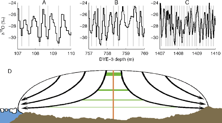Figure 1: Three 3-meter long sections (A-C) of annually resolved δ18O data from different depths of the 2,037 m long South Greenland DYE-3 ice core. The ages are (A) 175-180, (B) 1845-1854, and (C) 4657-4678 years before A.D. 2000, respectively. Gray bars show manually identified winter minima. (D) The ice flow leads to annual layer thinning that together with diffusion ultimately leads to a loss of the annual signal with depth.

Seasonal variations in isotopic composition and impurity content of the snowfall provide the basis for a distinct annual signal in the snowpack, which may be preserved in the ice under favorable conditions. The ability of an ice core to provide (sub-)annual information depends on the accumulation rate. It typically ranges from a few centimeters of ice per year in high-elevation areas of Antarctica to several meters at coastal sites of Greenland and on low latitude glaciers. In the upper part of an ice sheet, snow slowly compacts into incompressible ice. Due to the continuous accumulation of snow, annual layers become buried in the ice sheet over time. Gravity causes the ice to flow toward the ice sheet margins, which results in thinning of the annual layers with depth (Fig. 1). Close to the base of an ice sheet, ice flow over bedrock undulations causes folding and shearing leading to stratigraphic disturbances that can complicate precise dating of the lowermost section of an ice core.

Detecting the annual signal

The ratios of stable oxygen and hydrogen isotopes in glacier ice (expressed as δ18O and δD values) reflect seasonal variations in local temperature at the time of precipitation (Dansgaard 1964). In ice cores from high accumulation sites, such as the South Greenland DYE-3 core (Fig. 1), the seasonal signal may be traced 8,000 years back in time (Vinther et al. 2006). However, at lower accumulation sites, diffusion of water molecules during the transition from snow to ice reduces, or completely erases, the amplitude of the seasonal cycle. Moreover, ice flow-induced layer thinning and diffusion of water molecules within the deep ice ultimately obliterates the seasonal δ18O and δD cycles even in high-accumulation areas (Johnsen et al. 2000). Therefore, in deeper ice, other proxies less prone to diffusion must be employed for annual layer detection.

Figure 2: Example of continuous flow analysis data (smoothed curves in bold) from a shallow ice core from the North East Greenland Ice Stream (NEGIS) site. Several different impurities are measured, but here we show only the concentration of insoluble dust, Sodium ions, and Ammonium ions, chosen because the annual signal is expressed in different ways in these three data series. Manually identified winter layers (grey solid bars) and automated dating results (open gray bars; for method see Winstrup et al. 2012) agree in sections where the annual signal is clearly expressed in all three data series with a resolution sufficient to resolve even relatively thin layers.

An annual signal may also be preserved in the impurity content of an ice core, as many impurities display a seasonal variation (Fig. 2). In Greenland, for example, dust concentrations generally reach a maximum during spring, whereas the amount of sea-salt aerosols peaks during winter (Rasmussen et al. 2006). The annual dust cycle can sometimes be identified from the visible layering of an ice core (Svensson et al. 2005), but most impurity records are obtained by measurements on melted samples, often using a melting device and a high-resolution continuous flow analysis (CFA) system (Röthlisberger et al. 2000).

Counting of annual layers

In general, impurity records are more complex to interpret than isotope records as they also contain non-annual signatures, e.g. input from volcanic eruptions, biomass burning, and other episodic sources. For this reason, the parallel analysis of several impurity records of different origin is recommended when establishing a chronology. Extensive high-resolution CFA datasets have allowed for manual multi-proxy layer identification in ice cores from both hemispheres. In Greenland, data from several cores form the basis of the Greenland Ice Core Chronology 2005 (GICC05), which extends 60,000 years back in time (Svensson et al. 2008). Annual layers have also been identified back to ~30,000 years BP in the ice core drilled on the West Antarctic Ice Sheet Divide (WAIS Divide Project Members 2013), in the Antarctic EPICA Dronning Maud Land ice core (EDML), and in numerous younger ice cores from both hemispheres. These ice-core chronologies rely on manually identifying annual layers, which is laborious and inherently entails subjectivity. However, it is also a very flexible approach that can accommodate changes in the expression of annual layers, data quality, and resolution.

Development of new methods

New analytical techniques are widening the array of impurities that can be analyzed at annual resolution (McConnell et al. 2002). Moreover, refinement of CFA setups and data processing is increasing data resolution, now allowing detection of strata at the millimeter scale (Bigler et al. 2011). The resulting improvements in data quality and quantity allow for the extension and improvement of current ice-core chronologies as annual layers can now be detected in sections of the cores where annual layer identification has not previously been possible. Furthermore, development of new methods for statistical annual layer detection may soon supplement manual layer identification. Several automated approaches are being developed and have been applied to both single-record and multi-parameter data sets (Winstrup et al. 2012; Wheatley et al. 2012; McGwire et al. 2011). Among the more sophisticated approaches, the Bayesian algorithm by Winstrup et al. (2012) considers all possible divisions of a data series into an arbitrary number of layers, and selects the optimal division based on the appearance of layers and their individual thicknesses (Fig. 2). The method relies on assumptions of the statistical nature of the annual signal, the validity of which should be tested where independent dating methods allow for this. Providing that these assumptions are correct, the automated method produces objective annual layer-based ice-core chronologies with well-quantified uncertainties. Integrated uncertainty estimation is a key quality of this automated Bayesian method that represents a significant advance compared with manual subjective error estimates.

The accuracy-precision issue and new common chronological frameworks

As with any annually laminated record dated by layer counting, the uncertainty accumulates with increasing age. Consequently, the determination of absolute ages is very accurate for recent periods, while the accumulated uncertainty often becomes large (i.e. low accuracy) compared to e.g. radiometric dating uncertainties in the last glacial period. However, even when the absolute accuracy is relatively low, layer counting still provides the possibility to determine event durations as recorded in the ice cores very precisely. For example, the accuracy of the GICC05 time scale at the onset of the Holocene is about a century, while the outstanding precision allows for the analysis of how the transition into the Holocene is expressed in different proxy records with a maximum relative dating error of only a few years (Steffensen et al. 2008). In a similar way, the GICC05 counting uncertainty of a few percent in the glacial period makes it possible to constrain the duration of interstadial 11 in the Greenland record to 1100 years with a maximum counting error of just 54 years (high precision). In contrast, the absolute age of the event (43 ka before present) has a rather low accuracy due to an accumulated maximum counting error of 1700 years.

Ice cores from different sites can be synchronized using common time marker horizons of, for example, volcanic origin (Rasmussen et al. 2008; Severi et al. 2007; Parrenin et al. 2012) or common variations in methane levels (Blunier and Brook 2001; Pedro et al. 2011). Hence records from different sites can be aligned for parallel analysis with a precision that is often several orders of magnitude better than the absolute dating accuracy. Following this approach, the GICC05 chronology is currently being applied to all main Greenland ice cores to allow analysis of the climatic information from all cores in a consistent chronological framework. Recent studies also have employed a set of global event markers to synchronize ice cores from both hemispheres (Raisbeck et al. 2007; Svensson et al. 2013; Sigl et al. 2013) and are incorporating other sources of dating and ice flow information in a modeling framework in order to construct a consistent multi-ice-core chronology (Lemieux-Dudon et al. 2010). The fidelity of chronologies modeled that way increases with the addition of more data and better quantification of the entailing uncertainties (Veres et al. 2013; Bazin et al. 2013). However, annual layer counted sections have yet to be included in a way that respects the nature of the annual layer counting process and the involved uncertainty. Therefore, modeled chronologies following this approach must still be considered complementary to annual layer counted chronologies.

Experimental and analytic innovations keep pushing the construction of annual-scale ice-core chronologies forward. Upcoming developments may allow stratigraphic ice-core chronologies to reach further back in time, to reduce and better quantify uncertainties, and to become better integrated both regionally and on a global scale.

affiliation

Centre for Ice and Climate, Niels Bohr Institute, University of Copenhagen, Denmark

contact

Sune O. Rasmussen: olandergfy.ku.dk

references

Full reference list under: pastglobalchanges.org/products/newsletters/ref2014_1.pdf

Bazin L et al. (2013) Clim Past 9: 1715-1731

Bigler M et al. (2011) Environ Sci Technol 45: 4483-4489

Sigl M et al. (2013) J Geophys Res [Atmos] 118: 1151-1169

Svensson A et al. (2013) Clim Past 9: 749-766

Winstrup M et al. (2012) Clim Past 8: 1881-1895