PAGES Magazine articles

Antonietta Capotondi1, E. Guilyardi2 and B. Kirtman3

Some new exciting directions in ENSO research explore inter-event differences in spatial patterns, teleconnections and impacts, asymmetries between warm and cold phases, and the role of extra-tropical regions in triggering ENSO events. However, large uncertainties remain regarding ENSO projections.

The El Niño–Southern Oscillation (ENSO) is a naturally occurring fluctuation that originates in the tropical Pacific region and affects ecosystems, agriculture, freshwater supplies, hurricanes and other severe weather events worldwide. Over the last thirty years significant progress has been made in improving our understanding of the dynamic processes underlying ENSO, including the ocean-atmosphere feedbacks that are essential to this coupled phenomenon.

The oscillatory nature of ENSO, alternating between El Niño and La Niña events, can be described in terms of the recharge and discharge of warm water to and from the equatorial thermocline (“recharge oscillator”; Jin 1997) or in terms of thermocline depth changes associated with wave propagation (“delayed oscillator”, e.g. Suarez and Schopf 1988). These simple paradigms of ENSO as a linear oscillator capture basic dynamical processes; however, they fail to explain differences among events and asymmetries between warm and cold episodes. Moreover, they ignore the important role of stochastic atmospheric phenomena (e.g. westerly wind bursts) and other non-linear effects.

Understanding and predicting the diverse characteristics of El Niño and La Niña events is important since their regional climatic impact can vary heavily depending on the longitudinal location of the SST anomalies. Also, understanding how teleconnections vary depending on the event type is crucial when proxy records are used to reconstruct past ENSO. Hence, exciting new research developments have emerged to address this observed ENSO diversity.

Understanding ENSO dynamics

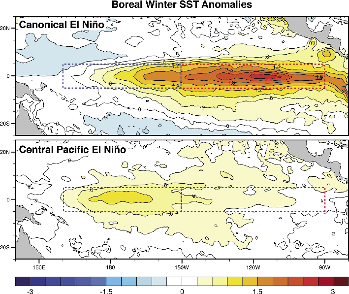
Figure 1: Composite spatial pattern of SST anomalies for the “canonical” (top) and “Central Pacific” (bottom) El Niño types (SODA 2.0.2/3) from 1958 to 2007 computed with the approach of Kug et al. (2009). Canonical El Niños are characterized by a boreal winter (DJF) Niño3 index larger than 0.5°C and larger than the Niño4 index (red and blue dashed boxes, respectively), and vice versa for the Central Pacific El Niño (from Capotondi, in press). Observed El Niño events can be described as blends of these two end-member types.

The first development is a renewed interest in inter-event differences and the related “El Niño Modoki” debate. Based on a statistical analysis of SST in the tropical Pacific, Ashok et al. (2007) suggested the existence of another type of El Niño, called Central Pacific El Niño (or Date Line El Niño or El Niño Modoki by various authors). They argued that this type of El Niño is not the same as the “canonical” El Niño because its center of action is in the central Pacific instead of the eastern Pacific, as illustrated in Figure 1. It was also suggested that Central Pacific El Niños have become more frequent in recent decades, and their frequency may increase further with global warming (Yeh et al. 2009). Subsequent observational and modeling studies have tried to define the Central Pacific El Niño more precisely or differently (Kug et al. 2009; Kao and Yu 2009). However, as yet no agreement has been reached on the best way to characterize the new Central Pacific-type of El Niño. Some studies have tried to distinguish the central Pacific and eastern Pacific (canonical) warm events based on their underlying dynamical processes, and their relationship with the oceanic mean state (e.g. Choi et al. 2011; McPhaden et al. 2011). A number of other studies dispute the statistical significance of the distinction between the two El Niño types or at least of the increasing occurrence of the Central Pacific variety. They argue either that the reliable observational record is too short to detect such a distinction (Nicholls 2008; McPhaden et al. 2011), or that they have found no trend using other approaches (Giese and Ray 2011; Newman et al. 2011; Yeh et al. 2011). Other authors alternatively suggest to distinguish between other types of El Niño, such as standard and extreme El Niños (Lengaigne and Vecchi 2010; Takahashi et al. 2011). Due to the asymmetric nature of the warm and cold phases of ENSO, Kug and Ham (2011) could not identify analogous distinctions for La Niña, neither in observations nor in the simulations of the Climate Model Intercomparison Project version 3 (CMIP3). Due to the large societal relevance of the impacts of ENSO, it is important to predict not only whether an El Niño (or La Niña) event is expected, but if possible which expression the anomaly will take. Fueled by these early studies, new questions are now emerging asking, for instance, if discrete classes of ENSO events emerge from observations, paleoclimate records and model simulations, or if ENSO diversity is better described as a continuum with a few characteristic extremes (e.g. Wu and Kirtman 2005).

Other new lines of research in ENSO diversity include revisiting the relative roles of the ocean and the atmosphere in shaping ENSO (Kitoh et al. 1999; Guilyardi et al. 2004; Dommenget 2010; Clement et al 2011; Lloyd et al. 2011) and exploring the role of regions outside the tropical Pacific in triggering ENSO events (Vimont et al. 2003; Izumo et al. 2010; Terray 2011; Wang et al. 2011). An example of remote influence is the seasonal footprinting mechanism (Vimont et al. 2003): Atmospheric variability originating in the North Pacific can impact the subtropical ocean during winter, and the resulting springtime SST anomalies alter the atmosphere-ocean system in the tropics during the following summer, fall and winter. The diversity of geographical sources and mechanisms proposed may explain the diversity of El Niño events, both in observations and in models.

ENSO in climate models and future projections

Most of our understanding of the representation of ENSO in climate models has been derived from the analysis of the model simulations of the Climate Model Intercomparison Project versions 3 (CMIP3) and 5 (CMIP5). While the models appear to reproduce some of the basic processes and feedbacks associated with ENSO, the details of the SST anomaly patterns as well as the temporal evolution of the anomalies often differ from the observed, and reflect model biases or erroneous atmosphere-ocean interactions (Capotondi et al. 2006, Guilyardi et al. 2009; Guilyardi et al. 2012a). For example, in most of the CMIP3 models, the largest anomalies are located further west along the equator than in observations. Furthermore, in many models ENSO events tend to occur more frequently and regularly than in the real world. While the models keep improving in their simulation of ENSO, no quantum leap was seen in CMIP5 compared against CMIP3 (Guilyardi et al. 2012b).

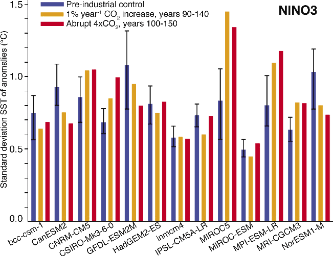
Figure 2: Standard deviation of Niño3 SST anomalies for thirteen CMIP5 model experiments. Blue bars, pre-industrial control experiments; orange bars, years 90-140 from the 1% year-1 CO2 increase experiments; red bars, years 50-150 after an abrupt four-fold CO2 increase. Model names are given on the x-axis. Error bars indicate the standard deviations over 50-year windows of Niño3 anomalies in the multi-century control experiments. Thus, when the Niño3 standard deviation in one of the CO2 runs falls outside the error bar, the changes are deemed significant (modified from Guilyardi et al. 2012b). As in CMIP3, this new set of model simulations does not provide a clear trend for ENSO strength in a warming climate.

Over the past few years, new promising methods have emerged, which could improve ENSO simulations, for example by bridging ENSO theoretical frameworks and climate modeling. Resulting innovations include the development of indices that can be used to assess the stability of ENSO in Coupled General Circulation Models (CGCMs), and intermediate models that can be used to predict ENSO characteristics from aspects of the mean state. By focusing on the key processes affecting ENSO dynamics (e.g. the thermocline feedbacks or the wind stress response to SST anomalies), these new approaches have much potential to accelerate progress and improve the representation of ENSO in complex climate models. Not only can these new methods help address the question of whether the characteristics of ENSO are changing in a changing climate, but potentially they can also improve the reliability of centennial-scale climate projections and predictions on seasonal time scales.

Looking forward

At present, we don’t know enough about how ENSO has changed in the past (the detection problem) and what caused the changes i.e. the contribution from external forcing vs. that due to internal variability (the attribution problem). Given the much too short reliable observational record (both for ENSO and for the external forcing fields, Wittenberg 2009), the complexity and diversity of the paradigms and processes involved, and the shortcomings of current state-of-the-art models, understanding the causes of ENSO property changes, both in the past and in the future, remains a considerable challenge. For instance Collins et al. (2010) concluded that it is not yet possible to say whether ENSO activity will be enhanced or damped in future climate scenarios, or if the frequency of events will change (Fig. 2). Paleoclimatic and paleoceanographic reconstructions have the potential to initiate the next quantum leap.

affiliations

1CIRES, University of Colorado, Boulder, USA; antonietta.capotondinoaa.gov

2LOCEAN, Institut Pierre Simon Laplace, Paris, France

3RSMAS/MPO, University of Miami, USA

Selected references

Full reference list online under: pastglobalchanges.org/products/newsletters/ref2013_2.pdf

Ashok K et al. (2007) Journal of Geophysical Research 112, doi:10.1029/2006JC003798

Capotondi A., Wittenberg A, Masina S (2006) Ocean Modeling 15: 274-298

Collins M et al. (2010) Nature Geoscience 3 (6): 391-397

Guilyardi E et al. (2009) Bulletin of the American Meteorological Society 90: 325-340

Guilyardi E et al. (2012a) Bulletin of the American Meteorological Society 93: 235-238

Diane M. Thompson1, T.R. Ault1, M.N. Evans2,1, J.E. Cole1,3, J. Emile-Geay4, A.N. LeGrande5

We use a simple proxy model to compare climate model simulations and coral records over the 20th century. While models and observations agree that the tropical oceans have warmed, they disagree on the extent and origin of freshening.

The response of the tropical Pacific Ocean to anthropogenic climate change remains uncertain, in part because we do not fully understand how the region has responded to anthropogenic change over the 20th century. Analysis of 20th century temperature and salinity trends is hindered by limited historical data, lack of long-term in situ measurements, and disagreement among coupled general circulation model (CGCM) hindcasts. High-resolution paleoclimate records, particularly the large network of tropical Pacific coral oxygen isotope records, are an alternate means of assessing tropical climate trends. However, these natural archives of past climate are biased by their limited spatial and temporal distribution and their biologically mediated response to climate. By converting native climate variables (e.g. temperature and net freshwater flux) into synthetic (“pseudo”) proxy records via an explicit proxy system model (“forward model”), we can directly compare historical climate data and climate model simulations with coral records, and assess biases and uncertainties associated with each.

Pseudocoral modeling

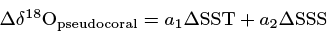
The stable oxygen isotope ratio (δ18O) of coral aragonite is a function of the temperature and the oxygen isotopic ratio of seawater (δ18Osw) at the time of growth; the latter is in turn strongly related to sea-surface salinity (SSS). As direct measurements of δ<18Osw are scarce, we model the expected δ18O anomalies of corals (δ18Opseudocoral) as a function of sea-surface temperature (SST) and salinity anomalies:

We define coefficient a1 as -0.22 ‰ ºC^-1 based on the relationship between temperature and the isotopic composition of the skeleton in well-studied coral genera (e.g. Evans et al. 2000). Coefficient a2 is estimated from basin-scale regression analysis of available observations of δ18Osw on SSS (LeGrande and Schmidt 2006; LeGrande and Schmidt 2011). Uncertainty in the application of the resulting bivariate model arises from the assumed independence and linearization of a1 and a2 and substitution of the second term for a direct dependence on δ18Osw.

We apply this simple forward model of δ18Opseudocoral to generate synthetic coral (pseudocoral) records from historical observations and CGCM simulations of temperature and salinity (Thompson et al. 2011). When driven with historical climate data, we found that this simple model was able to capture the spatial and temporal pattern of ENSO and the linear trend observed in corals from 1958 to 1990. Modeling pseudocorals with temperature and salinity individually also demonstrated that although warming accounts for the majority of the observed δ18Ocoral trend (60% of trend variance), salinity also plays an important role (40% of trend variance). The addition of the SSS term improved agreement between modeled pseudocoral and observed coral δ18O trends over pseudocoral trends modeled from SST only (Thompson et al. 2011).

20th century trends

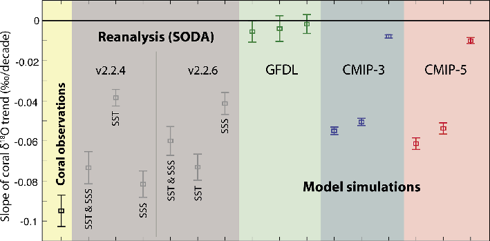
Figure 1: Magnitude of the trend slope (‰ per decade), computed by linear regression through the trend principal component (PC) in corals (far left) and pseudocorals modeled from Simple Ocean Data Assimilation (SODA) 20th century reanalysis (Carton and Giese 2008; Compo et al. 2011), a 500-year control run from the CGCM version CM2.1 of the Geophysical Fluid Dynamics Laboratory (GFDL cm2.1) (Wittenberg et al. 2009), and all CMIP-3 and CMIP-5 model ensembles (average of all models from each modeling group). In each case, δ18Ocoral was modeled from SST and SSS (1), SST only (2), and SSS only (3). Error bars depict ± 1 standard deviation of the regression estimate.

When driven with the output from 20th century simulations of a subset of CGCMs from the third phase of the Coupled Model Intercomparison Project (CMIP3) sampled at the coral locations, none of the pseudocoral networks reproduced the magnitude of the secular trend, the change in mean state, or the change in ENSO-related variance observed in the actual coral network from 1890 to 1990 (Thompson et al. 2011). Applying this same approach to the newer (CMIP5) suite of historical climate simulations, we find that large discrepancies still remain in the magnitude (Fig. 1), spatial pattern and ENSO-related variance of the simulated and observed trends. Differences between observed and simulated δ18Ocoral trends may stem from the simplicity of our forward model of δ18Ocoral, biological bias in the coral records, or model-inherent bias in the CGCM SST and SSS fields.

Although we cannot yet completely rule out a non-climatic origin for the amplitude of the observed δ18Ocoral trend, previous work highlights biases in simulated salinity fields as a potential source of the observed-simulated trend discrepancy (Thompson et al. 2011). We found that the suite of CMIP3 and CMIP5 CGCMs simulate weak and heterogeneous salinity trends that are indistinguishable in magnitude from that of unforced control runs (Fig. 1). Further, the pseudocoral simulations (Fig. 1) illustrate that the magnitude of the simulated δ18Ocoral trend can be less than the sum of the individual trends arising from temperature and salinity when the temperature and salinity trends are confounding at the coral sites (as observed for SODA modeled pseudocorals). However, given the limited number of historical SSS observations, much uncertainty remains in the sign and magnitude of the 20th century salinity trend. When forward-modeling pseudocorals with data from two recent versions of an extended reanalysis (SODA v2.2.4 and v2.2.6; Ray and Giese 2012), we found that even the relative contribution of temperature and salinity to the observed pseudocoral trend differs (Fig.1); this discrepancy likely arises from the choice of wind field used in the reanalyses (G. Compo, personal communication). These results suggest a need for improved simulation of moisture transport and additional proxy reconstructions of salinity and δ18Osw to better understand their relationship and the sign and magnitude of their change.

δ18Osw vs SSS: insights from isotope enabled simulations

Figure 3: Slope of the GISS ModelE2 simulated δ18Osw vs. salinity relationship at each gridbox on monthly (top) and decadal (bottom) timescales. Decadal series were calculated by averaging the monthly data at 10-year intervals.

In substituting the δ18Osw-SSS relationship calculated from the limited observational dataset for δ18Osw, our simple forward model assumes that this relationship is not only a valid approximation for δ18Osw, but also that this relationship does not vary significantly through time or within regions. Although this assumption does not likely hold at the millennial timescale (e.g. LeGrande and Schmidt 2011), it may be appropriate for simulating tropical variability during the past century. Here we assess the stability of the δ18Osw-SSS relationship through space and time on monthly to decadal timescales using a control simulation of an isotope-enabled version of the Goddard Institute for Space Studies model (GISS ModelE2, provided by A. LeGrande). In these simulations, the relationship between δ18Osw and SSS was generally regionally consistent over monthly to decadal timescales (Table 1), suggesting that the substitution of SSS for δ18Osw is unlikely to impose low-frequency variability on the modeled pseudocorals. However, we find that the slope of the δ18Osw-SSS relationship and its sensitivity to timescale varies within the broad regions of Table 1, particularly between the eastern and western Pacific (Fig. 2). Similar regional variability in the slope of the δ18Osw-SSS relationship was observed in an isotope enabled version of the UK Met Office model (HadCM3; Russon et al. 2013). Additionally, the slopes of the δ18Osw-SSS relationship simulated for the tropical regions in the GISS model were generally higher and more spatially consistent than those calculated from the limited observations (LeGrande and Schmidt 2006; Table 1). If we analyze only model output corresponding to the location and time of observations, the data-model discrepancy is reduced but not eliminated (Table 1). These discrepancies likely arise from the scarcity of paired δ18Osw and SSS observations as well as from the modeling of precipitation processes, and will be reduced by a combination of continued seawater sampling and model development.

If the current observational dataset underestimates the true magnitude of the δ18Osw-SSS slope, our simple forward model will underestimate the magnitude of the true δ18Ocoral trend when a significant freshening is observed. Estimates of uncertainty in the δ18Osw-SSS slope should be incorporated in future work simulating pseudocoral trends. Nonetheless, the salinity trend in CMIP3 and CMIP5 models is weak, and near zero, suggesting that the uncertainty in the δ18Osw-SSS relationship is not likely the source of the difference in the coral and pseudocoral trend magnitude. The presence of a significant freshening in historical observations suggests that this discrepancy is more likely due to an underestimation of the 20th century freshening in the CGCMs.

acknowledgements

We thank A. Wittenberg, B. Giese and G. Compo for contributing data and analysis products, and all those responsible for the PMIP3/CMIP5 simulation archives. Supported by NOAA’s Climate Change Data and Detection Program (NA10OAR4310115 to JEG, MNE, DMT; NA08OAR4310682 to JEC) and P.E.O International.

affiliations

1Department of Geosciences, University of Arizona, Tucson, USA; thompsodemail.arizona.edu

2Department of Geology and Earth System Science Interdisciplinary Center, University of Maryland, College Park, USA

3Department of Atmospheric Sciences, University of Arizona, Tucson, USA

4Department of Earth Sciences, University of Southern California, Los Angeles, USA

5NASA Goddard Institute for Space Studies and Center for Climate Systems Research, Columbia University, New York, USA

Selected references

Full reference list online under: pastglobalchanges.org/products/newsletters/ref2013_2.pdf

Evans MN, Kaplan A, Cane MA (2000) Paleoceanography 15(5): 551-563

LeGrande A, Schmidt G (2011), Paleoceanography 26, doi:10.1029/2010PA002043

LeGrande AN, Schmidt GA (2006) Geophysical Research Letters 33, doi:10.1029/2006GL026011

Russon, T, Tudhope AW, Hegerl GC, Collins M, and Tindall J (2013) Climate of the Past Discussions 9, 741-773

Thompson DM et al. (2011) Geophysical Research Letters, doi:10.1029/2011GL048224

Tom Russon1, A.W. Tudhope1, G.C. Hegerl1, M. Collins2 and J. Tindall3

Coral stable isotope records provide information on past ENSO variability. However, separating the contributions from variability in ocean temperature and the hydrological cycle to such records remains challenging. Model simulations using water isotope-enabled climate models provide powerful tools to explore this.

The stable oxygen isotopic composition of the aragonite of reef-dwelling corals (δ18Ocoral) relates to both the temperature, taken here as being the sea surface temperature (SST), and the isotopic composition of the seawater (δ18Osw) in which calcification occurred. The relationship between δ18Ocoral and SST, derived from modern calibrations, generally has a slope that is close to the value of -0.2‰ K-1 found for inorganically precipitated carbonates (e.g. Gagan et al. 2000; Zhou and Zheng 2003). Some long-lived corals generate sufficiently high growth rates as to allow measurement of δ18Ocoral at sub-annual resolution over multiple decades (e.g. Carré et al., this issue). These properties provide a strong basis for using fossil corals δ18Ocoral to reconstruct SST variability associated with the El-Niño Southern Oscillation (ENSO) over the Holocene and LGM (e.g. Tudhope et al. 2001; Cobb et al. 2003).

However, δ18Ocoral also depends directly on δ18Ocoral which is in turn influenced by a range of factors. Some of these factors may be closely coupled to ENSO, such as the local precipitation-evaporation balance, but others relate instead to the integrated hydrological history of the precipitation. In regions with a very active hydrological cycle, where the δ18Ocoral contribution is thought to dominate the overall δ18Ocoral signal, records have been used to infer past changes in precipitation, rather than SST (Cole and Fairbanks 1990). Fully quantifying the spatial pattern of relative contributions from SST and δ18Osw to δ18Ocoral remains a challenge for interpreting these records.

Limitations of the instrumental record

Instrumental records of δ18Osw are not available for most coral bearing locations and those that do exist are typically too short to allow robust quantification of inter-annual changes in δ18Osw (Schmidt 1999; LeGrande and Schmidt 2006). However, the δ18Osw contribution can be estimated empirically from an instrumental SST record, provided that (1) the ENSO-related δ18Osw fluctuations relate linearly to those in SST and (2) this relationship remains stationary throughout the period of interest. An example of a case in which the first assumption may be compromised is if the source region for precipitation changes with the magnitude of ENSO events. The second assumption may be compromised if the dominant spatial “modes” of ENSO variability change through time (Yeh et al. 2009; Capotondi et al., this issue). Climate model realizations of the response of δ18Osw to ENSO fluctuations have the potential to better constrain the validity of such assumptions.

Representing pseudo-corals in an isotope-enabled climate model

Only a few coupled Ocean/Atmosphere General Circulation Models (GCMs) include the additional hydrological cycle processes required to directly simulate water isotope variables such as δ18Osw. Modeling pseudo-coral records based on the use of δ18Osw proxy variables such as salinity, provide a strategy to avoid this limitation (Thompson et al. 2011, this issue). However, work with the isotope-enabled Goddard Institute for Space Studies ModelE-R shows that the slopes of the δ18Osw-salinity relationships may differ when calculated over temporal and spatial patterns of variability (LeGrande and Schmidt 2009). The results presented here are based on a 750-year long pre-industrial control simulation of another isotope-enabled coupled GCM, the UK Met Office’s HadCM3 (Russon et al. 2013; Tindall et al. 2009). The inter-annual variability of the tropical climate in HadCM3 is known to be dominated by processes exhibiting spatial and temporal patterns resembling, albeit with significant biases, those of the observed ENSO phenomenon (Collins et al. 2001; Guilyardi et al. 2006). For this study, the water isotope regimes were brought to equilibrium by first running the model for an additional 300 years from an assumed initialization state. The pseudo-coral δ18Ocoral field is then calculated directly by inputting the monthly-mean SST and δ18Osw data for the ocean grid resolution of 1.25º by 1.25º over the tropical Pacific (30ºS-30ºN and 120ºE-80ºW) into a linear formulation of the standard isotope paleo-temperature equation, with an assumed δ18Ocoral to SST slope of -0.2‰ K-1.

Quantifying the δ18Osw contribution

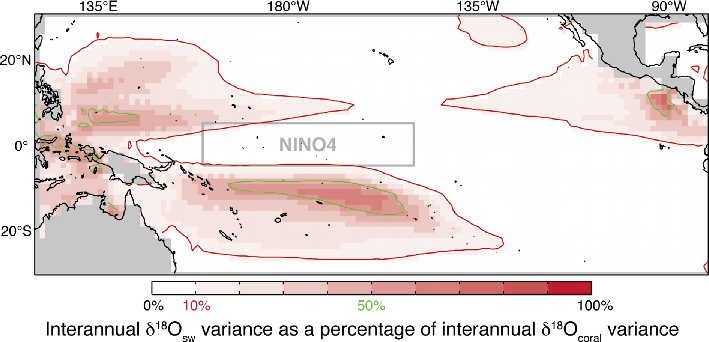
Figure 1: The percentage of modeled interannual δ18Ocoral variance accounted for by δ18Osw, assuming a SST - δ18Ocoral slope of -0.2‰ K-1. The 10% and 50% levels are contoured in red and green respectively and the location of the NINO4 region is highlighted in gray.

Modeled inter-annual fluctuations in δ18Osw vary inversely with those in SST across almost the entire tropical Pacific region such that they combine positively. The fraction of the inter-annual variance of pseudo-coral δ18Ocoral that could be accounted for by the inter-annual variance of modeled δ18Osw is less than 10% (red contour in Fig. 1) across much of the subtropical eastern and equatorial Pacific, but higher in the Warm Pool, South Pacific Convergence Zone, and central American coastal regions. This affirms that the δ18Osw contribution is indeed important in regions of high precipitation variability (Tudhope et al. 2001; Cole and Fairbanks 1990). Consequently, whilst eastern Pacific pseudo-coral δ18Ocoral could be reasonably used as a proxy of SST fluctuations, this is not the case for all locations. However, only in very limited regions does the δ18Osw contribution exceed 50% (green contour in Fig. 1). Even within the high precipitation regions, there are no locations where one would expect the SST contribution to be negligible. Therefore, interpreting western Pacific corals as solely (or even predominantly) dependent on either temperature or precipitation appears misguided for many locations in the model.

Non-linearity between SST and &delta18Osw

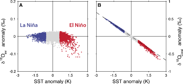
Figure 2: Scatter plots of modeled monthly inter-annual anomaly data within the NINO4 box. (A) δ18Osw plotted against SST. (B) δ18Ocoral plotted against SST, with the assumed slope of -0.2‰ K-1 used to calculate δ18Ocoral shown as a dashed line. Points are color coded according to their SST anomaly values, such that those lying in the upper and lower standard deviations of the SST data are highlighted red and blue, and are associated with El-Niño and La-Niña events respectively.

The regional relationships between modeled SST and δ18Osw are not always simple. For example, in the western equatorial Pacific NINO4 region (grey rectangle in Fig. 1), little relationship is seen between modeled SST and δ18Osw during La-Niña (blue crosses), neutral (grey crosses) and even moderate El-Niño (red crosses) regimes (Fig. 2a). This results in pseudo-coral δ18Ocoral values that lie close to the imposed δ18Ocoral-SST slope (Fig. 2b). In such situations, the δ18Osw variability effectively adds (a relatively small degree of) noise to the δ18Ocoral record. However, during larger El-Niño events a weak anti-correlation between SST and δ18Osw becomes evident (lower right quadrant of Fig. 2a), such that for SST anomalies exceeding ~1.5K, a deviation from the imposed slope of the δ18Ocoral-SST relationship becomes noticeable (lower right quadrant of Fig. 2b). For large El-Niño events, estimating NINO4 SST directly from δ18Ocoral would result in a relative overestimation of the true SST anomaly by over 20%. This effect would complicate attempts to accurately infer the relative magnitudes of the SST anomalies during El-Niño events of different magnitude from proxy records of δ18Ocoral alone.

acknowledgements

This work was funded by NERC grant NE/H009957/1

note

The model data presented here are available upon request from the corresponding author.

affiliations

1School of GeoSciences, University of Edinburgh, UK; tom.russoned.ac.uk

2College of Engineering, Mathematics and Physical Sciences, University of Exeter, UK

3School of Earth and Environment, University of Leeds, UK

Selected references

Full reference list online under: pastglobalchanges.org/products/newsletters/ref2013_2.pdf

LeGrande AN, Schmidt GA (2006) Geophysical Research Letters 33, doi:10.1029/2006GL026011

LeGrande AN, Schmidt GA (2009) Climate of the Past 5(3): 441-455

Russon T et al. (2013) Climate of the Past 9: 1543-1557

Thompson DM et al. (2011) Geophysical Research Letters 38, doi: 10.1029/2011GL048224

Tindall JC, Valdes PJ and Sime LC (2009) Journal of Geophysical Research 114, doi:10.1029/2008JD010825

P. Braconnot1 and Y. Luan1,2

Simulations suggest that Pacific interannual changes in sea surface temperature (SST) are smaller than SST seasonality, whereas the opposite is modeled for precipitation. Nonstationarity in ENSO patterns may affect the interpretation of past variability changes from climate records.

High-resolution paleoclimate indicators provide a unique opportunity to reconstruct and understand how seasonal climate variability and the El Niño-Southern Oscillation (ENSO) have evolved in the past. However, most climate interpretations of paleorecords assume stationarity, i.e. that the modern relationship between a given climate sensor and ENSO was the same in the past, which might not be true. Therefore, one of the difficulties is to infer how changes in mean state and variability have shaped the evolution of SST and other environmental factors, such as precipitation and wind, in the past. Using a suite of simulations performed with the climate model of the Institut Pierre Simon LaPlace (IPSL-CM4; Marti et al. 2010), we discuss the relative effects of different Holocene forcings on seasonality and interannual variability between the early Holocene and the pre-industrial period.

Sensitivity experiments

Previous simulations and model data comparison have established that long-term changes in insolation affected ENSO variability in the Holocene (Clement et al. 2000; Moy et al. 2002). However, the presence of melting remnant ice sheets in the northern hemisphere during the Early Holocene, may have partially offset the impact of the insolation forcing. In this study, simulations of the Early Holocene and the Mid-Holocene are used to infer how the slow variation of the Earth’s orbital parameters affected ENSO variability (Luan et al. 2012). We also conducted a set of sensitivity experiments to examine how meltwater release and the presence of remnant northern hemisphere ice sheets may have impacted ENSO characteristics (Braconnot et al. 2012; Marzin et al. in press). The different model years in the simulations were classified either as El Niño, La Niña, or normal years based on the December-January-February SST anomalies in the Niño3 region (150°W-90°W, 5°S-5°N). Anomalies were only classified as El Niño or La Niña events when they crossed a SST threshold of 1.2 times the standard deviation derived from the pre-industrial SST time series.

Figure 1: Composite sea surface temperature (SST) anomaly and precipitation anomaly maps during El Niño events as simulated by the IPSL-CM4 climate model for pre-industrial and Early Holocene (9.5 ka BP) climates. The anomalies describe the departures from normal years in each simulation at the peak of the event in December-January. Isolines are plotted every 0.5°C for SST with a refinement of 0.25°C around the 0 line, and every 1 mm d-1 for precipitation with a refinement of 0.5 mm d-1 around the 0 line. The red and blue dashed boxes in the lower left panel show the Niño3 and Niño4 regions, respectively.

ENSO is the dominant mode of SST and precipitation variability in all of the simulations. However, both the pre-industrial and past El Niño event simulations are affected by biases common to most climate models (Zheng et al. 2008). For example, the cold tongue (i.e. the equatorial region in the Pacific with cold SSTs) of normal years penetrates too far west along the equator (not shown), as does the equatorial warming associated with El Niño events (Fig. 1a,c). As a result the horseshoe structure of El Niño’s SST and precipitation patterns seen today in the western Pacific is not well pronounced. This discrepancy can lead to misinterpretation when comparing simulated changes with high-resolution coral records from the central equatorial Pacific region (Brown et al. 2008). In addition, simulations of ENSO variability are also damped in the eastern Pacific when compared with modern observations.

Spatial variability of ENSO patterns

Our simulations indicate that over time changes in forcing influence the location and intensity of the maximum SST and precipitation anomalies. In the Early Holocene for example, insolation forcing slightly damps the strength of the peak of the event (Fig. 1) compared with pre-industrial control simulations. In these Early Holocene examples a major reduction is simulated west of the maximum SST anomaly found in the pre-industrial control simulation, and another important reduction occurs on the South-American coast. Figure 1 therefore illustrates that the teleconnections between the different parts of the Pacific basin, as well as between the Pacific and the Indian Ocean, vary depending on the mean climate state. This further suggests that the climatic relationships between regions today are not stationary in time.

Changing seasonality and interannual variability accross time

Insolation forcing also affects the seasonality of SST and precipitation. Changes in the magnitude of the seasonal cycle of precipitation mirror the changes in the seasonal cycle of SSTs.

Figure 2: Sensitivity experiments: Diagrams of precipitation (mm d-1) averaged over the Niño3 and Niño4 regions in the Pacific Ocean. Groups of columns show the magnitude of the seasonal cycle and the peak (December) magnitude of El Niño and La Niña events for each of the simulations discussed in the text: pre-industrial (CTRL), Early Holocene (9.5 ka BP, EHnF), Early Holocene with a fresh water flux mimicking ice sheet melting in the North Atlantic (EHwF) and Early Holocene with the presence of remnant Laurentide and Fennoscandian ice sheets (EHIS). See Braconnot et al. (2012) for details on the methodology and statistical significance. The magnitude of the seasonal cycle is computed as the difference between maximum and minimum monthly values at the annual time scale. El Niño and La Niña anomalies correspond to the value at the peak of the event in December.

Figure 2 shows the Early Holocene insolation only simulations (EHnF), and pre-industrial control runs (CTRL) for two regions; the West (Niño4 region; 160°E-150°W, 5°S-5°N), and East (Niño3 region; 150°W-90°W, 5°S-5°N). Compared with the pre-industrial control run, the seasonal cycle of precipitation (“seas” in Fig. 2) was increased in the West (Niño4 region) and decreased in the East (Niño3 region) in the Early Holocene. These precipitation changes follow SST changes (not shown). It indicates that the seasonal variability in insolation was in phase with the SST seasonal cycle in the West and out of phase, in the East. The SST seasonal cycle is further amplified by the east-west asymmetry of cloud feedback and the dynamic response of SST to anomalous westerly winds in the eastern equatorial Pacific (Luan et al. 2012). As a consequence, seasonality had a larger effect on SSTs than do changes in interannual ENSO variability, even in the east Pacific (Braconnot et al. 2012).

With regards to precipitation, we note a reduction of larger absolute magnitude associated with El Niño and La Niña events in both the Niño3 and Niño4 regions when compared with the pre-industrial control runs (Fig. 2). Thus, both seasonality and interannual variability damp the SST and precipitation variations in the eastern Pacific, whereas seasonality enhance and variability damp precipitation in the central Pacific.

Our analyses have implications when interpreting records of past ENSO variability across different regions. In the eastern Pacific, Early Holocene seasonality and interannual SST and precipitation variability are reduced compared with SST and precipitation variability in the pre-industrial run. Therefore climate reconstructions, which are primarily determined by the relative sensitivity of climate sensors to seasonality and interannual variability, must take this into account in their calibrations in order to derive robust reconstructions.

In the central to western part of the basin, changes in seasonality and interannual variability act in opposite directions, and our results suggest that only the natural archives that are sensitive to precipitation would register large ENSO changes in the Early Holocene.

Role of additional forcings

The addition of a fresh water flux in the North Atlantic in the Early Holocene simulations leads to increased interannual variability and a slight increase in seasonality (Fig. 2; EHwF) compared with the simulation in which only insolation is changed (Fig. 2; EHnF). This suggests the fresh water flux partially offsets the changes due to insolation compared with the pre-industrial simulation (Fig. 2). This result is similar to the results of fresh water flux experiments under modern (Timmermann et al. 2007) or glacial (Merkel et al. 2010; see also Merkel et al., this issue) conditions. The presence of ice sheets (Fig. 2; EHIS) in the simulations, leads to a strong reduction in seasonality and a further damping of interannual precipitation variability compared with the insolation-only simulation. Particularly in the western Pacific, the results suggest that the remnant ice-sheets in the Early Holocene may have offset the amplification of precipitation seasonality.

Towards a better understanding

Our results show that the pattern of ENSO anomalies between the east and west Pacific is affected differently by forcings, but that SST variations during the Holocene were predominantly influenced by changes in seasonality driven by the Earth’s orbital parameters such as insolation.

Linking the development of an El Niño event with changes in the seasonal evolution of the thermocline depth is a key factor explaining the damping of the simulated ENSO in the IPSL models (Luan et al. 2012). Our sensitivity experiments show that fresh water fluxes partially counteract the insolation-driven seasonal phasing and the melting remnant ice sheets strongly affect the mean thermocline depth and east-west gradient in SSTs (Luan et al. submitted). However, it seems that precipitation and SSTs do not necessarily vary with the same relative strength on seasonal and interannual timescales when subject to the same sensitivity experiments. These findings suggest that a better understanding of the controls and timescales of variability is necessary to interpret paleo-records of past ENSO variability correctly, and that paleo-records should be used with caution to test how well models reproduce changes in ENSO variability.

affiliations

1Laboratoire des Sciences du Climat et de l’Environnement, Gif-sur-Yvette, France; pascale.braconnotlsce.ipsl.fr

2State Key Laboratory of Numerical Modeling for Atmospheric Sciences and Geophysical Fluid Dynamics, Institute of Atmospheric Physics, Beijing, China

Selected references

Full reference list online under: pastglobalchanges.org/products/newsletters/ref2013_2.pdf

Braconnot P, Luan Y, Brewer S, Zheng W (2012) Climate Dynamics 38: 1081-1092

Clement AC, Seager R, Cane MA (2000) Paleoceanography 15(6): 731-737

Merkel U, Prange M, Schulz M (2010) Quaternary Science Reviews 29(1-2): 86-100

Luan Y et al. (2012) Climate of the Past 8: 1093-1108

Zheng W et al. (2008) Climate Dynamics 30: 745-762

Claire E. Lazareth1, M.G. Bustamante Rosell1, N. Duprey1, N. Pujol2, G. Cabioch1,§, S. Caquineau1, T. Corrège2, F. Le Cornec1, C. Maes3, M. Mandeng-Yogo1 and B. Turcq1

“Seasonal amplitude was higher in the Southwest Pacific during the mid-Holocene,” say the corals. “It was not,” reply the models. “More work is needed,” agree the researchers…

In the Southwest (SW) Pacific, the seasonal changes in seawater surface characteristics, such as temperature (SST) and salinity (SSS), are governed mainly by the position and intensity of the South Pacific Convergence Zone (SPCZ) and by the occurrences of El Niño and La Niña events. The SPCZ is a southeast narrow cloudy belt that influences the wind and rain conditions from Papua New Guinea to French Polynesia (Trenberth 1976). During the austral summer, the SPCZ moves southwest whereas during the austral winter it moves north. Consequently, waters in the SW Pacific are generally warmer and less saline during the austral summer, and colder and saltier in winter. At the interannual time scale, the main changes in SST and SSS in the SW Pacific relate to El Niño-Southern Oscillation (ENSO) dynamics, with a periodicity of ca. 2-7 years (Trenberth 1976). During an El Niño event, warm waters of the equatorial West Pacific (the Warm Pool) and connected precipitation migrate toward the central and eastern Pacific. Consequently, the SW Pacific SST decreases slightly while precipitation decreases strongly, leading to higher SSS (e.g. Delcroix 1998). The opposite occurs during La Niña events. Therefore, knowledge of past water characteristics at a seasonal resolution has the potential to provide information on the position and intensity of the SPCZ as well as on the occurrence of ENSO events. Mid-Holocene (6 ka BP) hydrographic proxy data from the SW Pacific are rare. However, this is a key period, characterized by a change in ENSO amplitude that is unfortunately not yet entirely understood.

Corals and numerical models: tools to look back in time

Past seasonal data on SST and SSS can be obtained from archives such as massive coral skeletons. The aragonitic skeleton of coral is secreted by polyps over several decades or centuries, at a rate of around 1 cm year-1 for massive forms. The chemical composition of skeletal aragonite reflects the properties of the water in which the coral has lived. In tropical areas, studies focus on the massive Porites sp. corals. The Strontium/Calcium (Sr/Ca) ratio (Corrège 2006) is a robust proxy for SST in these corals. The stable oxygen isotopic ratio (δ18O) is used, combined with Sr/Ca, to reconstruct the isotopic composition of surface seawater (δ18Osw), which is in turn closely related to SSS (via the evaporation vs. precipitation budget).

Climate models, based on current knowledge of the various compartments of the Earth system, help understand modern climate variability and predict future changes. Climate models with external forcings different to current ones (e.g. different orbital forcings, ice sheets, greenhouse gas concentrations) can be used to simulate past climatic changes. Many model simulations exist for the mid-Holocene (e.g. 19 in the Paleoclimate Modelling Intercomparison Project [PMIP2] database; http://pmip2.lsce.ipsl.fr/; Braconnot et al. 2007). Their main forcing is a millennial-scale change in the seasonality of insolation. For the SW Pacific region, the insolation for January to March was lower than at present while it was higher for August to October.

To gain an insight into SW Pacific mid-Holocene mean climate at seasonal resolution and hence into ENSO characteristics, we studied corals from New Caledonia and Vanuatu which have been dated to 5.5 ka BP and 6.7-6.5 ka BP respectively. A ~1 cm-thick slab, cut along the axis of maximum growth of the coral colonies, was X-rayed to reveal the annual growth bands. To ensure the skeleton was well preserved, pieces were collected and analyzed for their mineralogy using X-ray diffraction, and for their microstructure using scanning electronic microscopy. If the skeleton preservation was found to be satisfactory, the slab was continuously sampled at 1-mm steps, providing on average one sample per month of coral growth. The samples were then dissolved and analyzed to determine their chemical composition. The New Caledonia coral was too short (~20 years) to investigate ENSO dynamics and as the δ18O proved to be partly altered, only the SST reconstructed with Sr/Ca will be discussed here.

The 6 ka BP PMIP2 model simulations show a cooling of the tropical Pacific SST (Zheng et al. 2008) and a decrease in seasonal SST amplitude (south of 10°S and between 160-260°E for the South Pacific) related to the insolation change. The results obtained on the New Caledonia coral were compared with the six simulations for which monthly data were available and which correctly reproduced the current SST cycle in the New Caledonia region on four 2° by 2° grid points (164-168°E, 20-24°S).

The SPCZ at 6 ka BP: Where was it located?

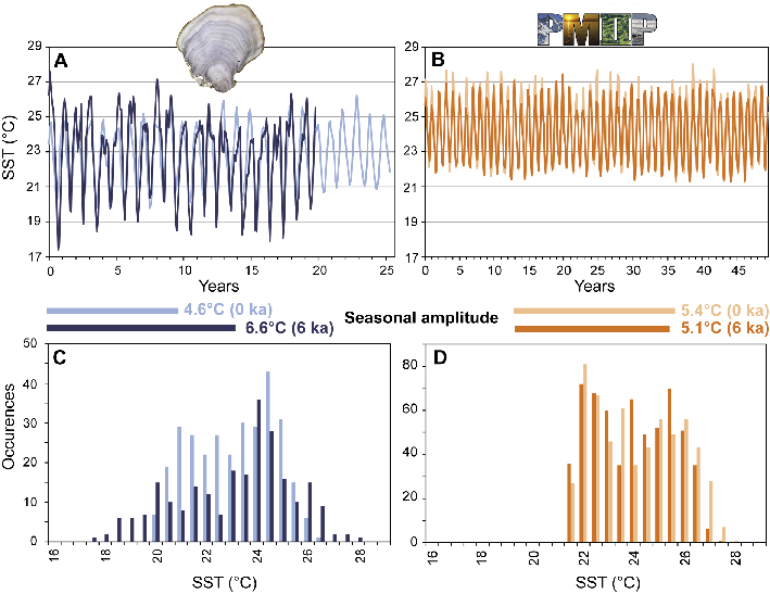
Figure 1: Comparison between coral (blue) and model run (orange) results in terms of sea surface temperature (SST; °C) characteristics in the New Caledonia region for the present (light colors) and the mid-Holocene (dark colors) situations. (A) Monthly coral time series from New Caledonia, at present (light blue, Stephans et al. 2004; Stephans et al. 2005) and from a coral fossil from the mid-Holocene (5.5 ka BP, dark blue; Lazareth et al. 2013). (B) Monthly time series from the CCSM PMIP2-models for the New Caledonia region (160-164°E 20-24°S), at present (light orange) and at the mid-Holocene (6 ka BP; dark orange; Otto-Bliesner et al. 2006). C, D) Monthly SST histograms and calculated seasonal amplitude.

In the New Caledonia lagoon, the mid-Holocene SST seasonal amplitude as seen by the corals was higher than nowadays (Fig. 1a). This difference is mainly due to colder mid-Holocene winters. In the New Caledonia region, the histogram of both the modern and mid-Holocene coral-reconstructed SST monthly values (Fig. 1c), and the 0 ka BP model outputs (Fig. 1d) show two modes, corresponding to the positions of the SPCZ in winter (July-August-September, JAS) and in summer (December-January-February, DJF). In the 6 ka BP coral results however, colder temperatures prevail in the winter mode, with a wider distribution. We interpret this as reflecting a more variable position and/or a weakening of the SPCZ during mid-Holocene winters. None of the PMIP2 models for the New Caledonia region reproduce an increase in seasonal SST amplitude in the mid-Holocene and the bi-modality is maintained (Fig. 1d). The models generally follow the insolation change: a warmer winter and a colder summer, leading to reduced seasonality (Fig. 1b).

For the Vanuatu corals, Sr/Ca and δ18O were measured as proxies for SST and SSS, respectively, and data from the longest colony were used to highlight ENSO characteristics during the early mid-Holocene. The precipitation regime in Vanuatu at 6.7-6.5 ka BP was different from the current one. Fossil corals indicate peaking SSS in summer (DJF) whereas low SSS would have been expected from the reduced summer insolation at that time. Indeed, summer today is accompanied by strong precipitation brought by the southward displacement of the SPCZ. The reconstructed high mid-Holocene SSS suggests that in the SW Pacific at 6.7-6.5 ka BP the SPCZ was located further north than nowadays (Duprey et al. 2012). At that time, ENSO variability was reduced by 20-30% compared to the modern ENSO. It remains uncertain, however, whether the reduced ENSO variability reflects a real trend in ENSO dynamics or if it resulted from a weaker coupling between the precipitation regime and the SPCZ.

Are proxy data and models compatible for 6 ka BP?

Figure 2: Multi-model mean maps for the winter season (July-August-September, JAS). Six PMIP2 simulations having similar resolution and reproducing correctly the mean seasonal cycle in the New Caledonia region have been used. The arrow points to New Caledonia. (A) SST multi-model maps at 0 ka (left) and difference (6 ka – 0 ka; right). (B) Multi-model mean precipitation field at 0 ka (left) and 6 ka (right). Modified from Lazareth et al. (2013).

While coral records suggest a reduced SPCZ influence in the SW Pacific, possibly from 6.7-6.5 to 5.5 ka BP, the PMIP2 model maps of precipitation reveal only a small shift of the SPCZ towards the northeast and a decrease in associated precipitation during the winter months (Fig. 2b). These small changes, although in the right direction, are, however, not sufficient to simulate an increase in the SST seasonality in the SW Pacific region at 6 ka BP.

The modeled insolation-driven hemispheric change in seasonality is not reflected in the SW Pacific proxy data. This suggests the models have difficulty in reproducing mid-Holocene changes in coupled ocean-atmosphere circulation in this region. This could be due to known model biases in representing the current, and thus also the 6 ka BP, SPCZ, and to the models’ large grid size to which the SPCZ seasonal displacement is sensitive. On the other hand, corals are shallow water organisms and the SST and SSS they record may not be valid for open oceans. Clearly, more data and new model runs are needed to understand the amplitude and geographical pattern of western Pacific mid-Holocene changes.

affiliations

1IPSL/LOCEAN, UPMC/CNRS/IRD/MNHN, Institut de recherche pour le développement France Nord, Bondy, France; claire.lazarethlocean-ipsl.upmc.fr

2University of Bordeaux, Environnements et Paléoenvironnements Océaniques et Continentaux, Talence, France

3Laboratoire d’Etudes en Géophysique et Océanographie Spatiales, Institut de Recherche pour le Développement, Toulouse, France

§To Guy, in memoriam

Selected references

Full reference list online under: pastglobalchanges.org/products/newsletters/ref2013_2.pdf

Braconnot P et al. (2007) Climate of the Past 3: 261-277

Corrège T (2006) Palaeogeography Palaeoclimatology Palaeoecology 232: 408-428

Delcroix T (1998) Bulletin de l'Institut Français d'Etudes Andines 27: 475-483

Duprey N et al. (2012) Paleoceanography 27, doi:10.1029/2012PA002350

Trenberth KE (1976) Quarterly Journal of the Royal Meteorological Society 102: 639-653

Ute Merkel, M. Prange and M. Schulz

Simulations of the climate of Marine Isotope Stages 2 and 3 suggest pronounced ENSO variability during the Heinrich Stadial 1 period when the Atlantic overturning circulation was weaker. Our model results also highlight the nonstationarity of ENSO teleconnections through time.

A well-known example of coupled ocean-atmosphere interaction on interannual timescales is the El Niño-Southern Oscillation (ENSO) phenomenon in the tropical Pacific. Consensus is still lacking about how ENSO will behave under future climate conditions, even in the latest generation of comprehensive climate models (Guilyardi et al. 2012).

Major goals of paleoclimatic research are to provide constraints on the possible range of changes in response to modified boundary conditions and to identify possible feedback and amplification mechanisms in the climate system. In this context, climate models are valuable tools for investigating different climate scenarios that have occurred in the past. Most ENSO studies, however, are limited to the two priority periods specified by the Paleoclimate Modeling Intercomparison Project (PMIP): the Mid-Holocene, and the Last Glacial Maximum (LGM; e.g. Zheng et al. 2008). However, proxy data from the tropical Pacific (e.g. Stott et al. 2002; Leduc et al. 2009; Dubois et al. 2011) suggest that ENSO also changed on millennial timescales, e.g. in association with pronounced abrupt climate changes related to the Dansgaard-Oeschger stadials and interstadials during Marine Isotope Stage 3 (MIS3, 59-29 ka BP).

Modeling ENSO for different glacial climate states

The first modeling studies that addressed MIS3 were limited to intermediate complexity models (e.g. Ganopolski and Rahmstorf 2001; van Meerbeeck et al. 2009; Ganopolski et al. 2010), a regional model approach (e.g. Barron and Pollard 2002), or an atmosphere-only setup (Sima et al. 2009), unsuitable to capture the complexity of ENSO dynamics. Recently, the first simulations of MIS3 climate in a comprehensive coupled climate model were accomplished with the US National Center of Atmospheric Research's CCSM3 model (Merkel et al. 2010). The study used a timeslice approach with a focus on a period of relatively regular Dansgaard-Oeschger variability around 35 ka BP. When 35 ka BP boundary conditions (greenhouse gas concentrations, orbital parameters, continental ice sheet distributions) are prescribed, the model simulates a very weak Atlantic meridional overturning circulation (AMOC) of about 7 Sv, which is much weaker than the preindustrial value of 12 Sv, but also weaker than the ~10 Sv simulated for the LGM. Therefore, we consider the simulated 35 ka BP climate as a stadial climate state. The counterpart of an interstadial climate state is induced in the model by a 0.1 Sv freshwater extraction from the North Atlantic over ~300 model years, thereby forcing a resumption of the AMOC to ~14 Sv.

Our set of experiments also includes a simulation of a Heinrich Stadial 1 scenario. This is set up by imposing a freshwater perturbation of about 0.2 Sv to a simulated LGM ocean state over 360 model years. This is motivated by earlier studies which mimic past Heinrich events by hosing freshwater into the modern ocean and thereby demonstrate that a slowdown of the AMOC may have a pronounced impact on the tropical Pacific (e.g. Timmermann et al. 2007).

Figure 1: ENSO variability of sea surface temperature in the eastern tropical Pacific (Niño3 region: 150°W-90°W, 5°S-5°N) for different simulated climatic states.

One of our major findings was that interannual (about 1.5-8 years) variability in sea surface temperatures (SST) of the eastern tropical Pacific was distinctly increased in our Heinrich Stadial 1 simulation compared to pre-industrial times, whereas variability in our LGM and MIS3 simulations was systematically reduced, albeit only weakly (Fig. 1). Modern ENSO dynamics studies show that stronger ENSO variability is dynamically linked to a weaker annual cycle of SST and to a weaker meridional asymmetry of SST across the equator in the eastern tropical Pacific (Guilyardi 2006; Xie 1994). Our model results show that these relationships also hold for the different simulated glacial climate states. In particular, our Heinrich Stadial 1 simulation exhibits a much weaker north-south contrast in eastern tropical Pacific SST than under modern conditions. This is attributed to an atmospheric signal communication from the strongly cooled North Atlantic into the tropical Pacific.

Model-data comparison

Further insights into tropical Pacific variability can be achieved through model-data intercomparison. Felis et al. (2012) present findings from a fossil coral retrieved during IODP Expedition 310 near Tahiti. The coral has been dated to Heinrich Stadial 1. Its fast growth rate allows sampling at monthly resolution and provides a unique opportunity to investigate interannual SST variability in the southwestern tropical Pacific during that period. The coral record exhibits pronounced variability at interannual ENSO frequencies during Heinrich Stadial 1, consistent with the basinwide increase in ENSO variability in our Heinrich Stadial 1-analogue simulation. At the Tahiti location, the coral and the model are also quantitatively consistent, as both suggest a strengthening of interannual SST variability by 20-30% compared to modern conditions.

Modern and past ENSO teleconnections

Figure 2: ENSO teleconnections during boreal winter (Dec.-Feb.): El Niño minus La Niña composites of sea level pressure [hPa] for (A) pre-industrial control climate, (B) Last Glacial Maximum (LGM), and (C) Marine Isotope Stage 3 (MIS3) stadial climate. Figure modified from Merkel et al. 2010.

Modern ENSO is well known for its atmospheric teleconnections of near-global extent. Understanding how teleconnections operate, both in the atmosphere and the ocean, is particularly relevant for the validity of paleoclimatic reconstructions, as they generally assume that atmospheric teleconnection patterns are stable. This may be particularly critical in the interpretation of proxy records not stemming from the core ENSO region. A composite analysis of atmospheric patterns (e.g. of sea level pressure) during all El Niño and La Niña events in the different simulations revealed obvious deviations from the modern spatial distribution of anomalies (Fig. 2). In particular, the teleconnections to the North American continent and the North Atlantic region seem to be strongly altered in terms of amplitude and spatial structure in the LGM and MIS3 simulations. This difference is probably caused by the presence of the glacial continental ice sheets and the glacial cooling of the North Atlantic, which both affect the position of the upper-tropospheric jetstream and atmospheric storm tracks, and thus the tropical-extratropical signal propagation. The typical intensification of the Aleutian low forced by El Niño (Fig. 2a) seems to be present during the LGM but is less pronounced, and the atmospheric bridge to the North Atlantic region seems to be interrupted, as no clear large-scale pattern is simulated there (Fig. 2b). The MIS3 stadial conditions (Fig. 2c) bear more resemblance to the control simulation over the North Pacific, whereas over the North Atlantic, the ENSO influence is clearly reduced, similar to the LGM situation. This points to a complex interplay of atmospheric dynamics with the various forcings in the different climatic states.

The need to learn more about glacial climatic states

In summary, our modeling study confirms that ENSO variability responds to various glacial climatic states. However, ENSO variability does not appear to be linearly linked to the strength of the AMOC. This calls for more detailed analyses, for instance in the form of glacial hosing studies in a multi-model approach (Kageyama et al. 2013). The different roles of the AMOC and the various glacial boundary conditions with respect to their impact on ENSO need to be further disentangled. Likewise, we emphasize that the concept of stationary teleconnections should only be applied to past climatic states with caution as they may be altered by different past boundary conditions and forcings internal and external to the climate system.

affiliation

MARUM - Center for Marine Environmental Sciences, University of Bremen, Germany; umerkelmarum.de

Selected references

Full reference list online under: pastglobalchanges.org/products/newsletters/ref2013_2.pdf

Felis T et al. (2012) Nature Communications 3, doi:10.1038/ncomms1973

Guilyardi E et al. (2012) CLIVAR Exchanges 58(17): 29-32

Kageyama M et al. (2013) Climate of the Past 9: 935-953

Merkel U, Prange M, Schulz M (2010) Quaternary Science Reviews 29: 86-100

Zheng W et al. (2008) Climate Dynamics 30: 745-762

Chris Brierley

The Pliocene was characterized by a weak equatorial sea surface temperature gradient in the Pacific, confusingly reminiscent of that seen fleetingly during an El Niño. Data also show interannual variability in the Pliocene, raising questions about ENSO’s dependence on the mean climate state.

The behavior of the El Niño–Southern Oscillation (ENSO) in pre-Pleistocene climates is highly uncertain. This uncertainty is rooted in a fundamental lack of evidence. However, several, recent studies focusing on past warm climates are beginning to address this issue. These studies were motivated by suggestions that the climate of the early Pliocene was a “permanent El Niño” – a term that has led to much confusion. After looking at the new evidence for ENSO, I will discuss the history of the term “permanent El Niño”, before suggesting that it should be consigned to history as well.

Pre-Pliocene ENSO

Detection of interannual variability requires paleoclimate indicators that monitor changes over short timescales such as the thickness of varved sediments and isotope ratios in long-lived fossil mollusks or corals. Once a record spanning sufficient years has been recovered, its power spectra can be analyzed for frequencies representative of ENSO. ENSO has been detected during the warm intervals of the Miocene (5.96-5.32 Ma; Galeotti et al. 2010), Eocene (45-48 Ma; Huber and Caballero 2003; Lenz et al. 2010) and Cretaceous (70 Ma; Davies et al. 2011, 2012) from layered deposits or varved sediments showing a strong peak in the 3-5 years range. It has also been seen in the Eocene (50 Ma; Ivany et al. 2011) from analysis of power spectra of carbon isotopes in fossil driftwood and bivalves. All of these analyses have used records gathered in locations far away from the tropical Pacific, such as Antarctica. However, ENSO teleconnections depend on the mean climate state (Merkel et al., this issue) and may therefore have been different in these early warm periods. The plausibility of assumed teleconnections of that time can be confirmed with climate model simulations of the period (Galeotti et al. 2010; Huber & Caballero 2003; Ivany et al. 2011).

Pliocene ENSO

Figure 1: Variation in the Sea Surface Temperature in the Equatorial Pacific over the past five million years. The estimates come from two ocean cores in the West (ODP 806 at 150°E) and the East (ODP 847 at 95°W). Two different types of record are used to reconstruct the temperatures: Mg/Ca (Wara et al. 2005) and alkenones (Dekens et al. 2007; Pagani et al. 2010). The period described as lacking ENSO variability (i.e. the period of the “permanent El Niño”) from a mistaken interpretation of Fedorov et al. (2006) is shown in orange. Times with observed ENSO variability, as found by Scroxton et al. (2011) and Watanabe et al. (2011), are marked in green. The time-slab used by PlioMIP and its precursors is marked as “mPWP”. Figure modified after Fedorov et al. (2013).

Two studies have found evidence of ENSO-style periodicity during the Pliocene (Fig. 1) from locations in the Tropical Pacific. Oxygen isotope records from fossil corals (MacGregor et al., this issue) from the Philippines show power spectra similar to recent corals, hence likely representing ENSO variability (Watanabe et al. 2011). Analyses of individual foraminifera from the Eastern Equatorial Pacific (Scroxton et al. 2011) find several instances of isotopic compositions outside the range predicted for the present-day seasonal cycle. This has been interpreted as showing an active ENSO cycle. Unfortunately, a foraminifer does not live through an annual cycle (unlike mollusks; e.g. Carré et al., this issue), so changes in the seasonal cycle (Braconnot and Luan, this issue) are a potential source of uncertainty.

Despite the complications associated with each individual study, a picture is emerging in which ENSO is a pervasive feature of past climate. However, a systematic effort will be needed to provide quantitative information from these pre-Pliostocene intervals that could qualify for data-model comparisons.

The “permanent El Niño” of the Early Pliocene

One of the factors fuelling the hunt for ENSO in pre-Pleistocene warm climates was the idea that the early Pliocene was in state of “permanent El Niño”. Mg/Ca records (a proxy for sea-surface temperatures, SST) from the Western and Eastern Equatorial Pacific (Wara et al. 2005) suggest that no temperature gradient existed along the equatorial Pacific around four million years ago (4 Ma; Fig. 1). Subsequent work shows similar results for the equatorial SST gradient in the early Pliocene. Reconstructions of the SST gradient during older periods need further work, but preliminary data suggest that a reduced SST gradient is not solely a feature of the early Pliocene (LaRiviere et al. 2012) although it may not be a ubiquitous feature of all warm climates (Nathan and Leckie 2009).

An El Niño event (the warm phase of the ENSO oscillation) is characterized by a lack of SST gradient along the equatorial Pacific. Although Wara et al. (2005) emphasized that their Mg/Ca records reflected the mean climatic state, i.e. a change in the long-term average climate rather than a change in interannual variability, they described their observation using the shorthand of “a permanent El Niño”. The term was propagated by Fedorov et al. (2006), who used model simulations to examine how such a state could be maintained. They emphasized the similarity between the long-term average state and the conditions seen during recent El Niños. This simile has been read as an assertion that there was no ENSO variability before 3 Ma, although this is not what the authors intended (Alexey Fedorov, personal communication) and is certainly not what is shown by the more recent studies described above.

Equatorial SST gradient and ENSO in models

The mid-Pliocene warm period (3.3-3.0 Ma; marked “mPWP” in Fig. 1) has been the focus of sustained effort by the data and modeling communities, most recently under the auspices of the Pliocene Model Intercomparison Project (PlioMIP; Dolan et al. 2012). This period is one million years later than the minimal SST gradient identified by Wara et al. (2005), but is thought to share similar climate forcings (Fig. 1). Haywood et al. (2007) found ENSO variability in both mid-Pliocene and modern simulations. However, the equatorial temperature gradient of the mid-Pliocene simulation was hardly smaller than in the modern simulation. Subsequent simulations performed with updated boundary conditions (Dowsett et al. 2010), similarly show a lack of strong reductions in the equatorial temperature gradient between the mPWP and the modern day (Haywood et al. 2013) – in comparison with the halving seen in the paleo-observations (Fig. 1).

Figure 2: Niño 3.4 SST anomalies in two model simulations; a control (green) and one with an equatorial SST gradient that is approximately halved (red). The shaded area represents four standard deviations from a 30-year running window (Fedorov et al. 2010).

Attempts have been made to force coupled models to replicate a mean state with a weak SST gradient in the equatorial Pacific. One approach has been to increase the background ocean vertical diffusivity (Brierley et al. 2009), potentially to represent a changed tropical cyclone distribution (Fedorov et al. 2010). These simulations (Fig. 2) appear to show a relationship between equatorial SST gradient and the amplitude of ENSO, but not its period (Fedorov et al. 2010). This result could easily be model dependent, but offers a scenario for a weak ENSO around 4.2 Ma, the time for which proxy data suggest that the SST gradient was very small (open orange box in Fig. 1).

Conclusion

The introduction of the term “permanent El-Niño” in the literature has caused confusion, but it has also motivated paleoclimatologists to look for (and find) evidence of interannual ENSO variability in deep time. The assertion that there was no ENSO variability before 3 Ma, wrongly attributed to Fedorov et al. (2006), is not true. However, the relationship between a Pacific mean state with a minimal equatorial SST gradient and related ENSO properties merits further investigation. We have made progress towards uncovering ENSO behavior on geologic timescales, but there is still a long way to go.

affiliation

Department of Geography, University College London, UK; c.brierleyucl.ac.uk

Selected references

Full reference list online under: pastglobalchanges.org/products/newsletters/ref2013_2.pdf

Fedorov A, Brierley C, Emanuel K (2010) Nature 463: 1066-1070

Fedorov A et al. (2006) Science 312: 1485-1489

Scroxton N et al. (2011) Paleoceanography 26(2), doi: 10.1029/2010PA002097

Wara MW, Ravelo AC, Delaney ML (2005) Science 309: 758-761

Watanabe T et al. (2011) Nature 471: 209-211

Gregory J. Hakim1, J. Annan2, S. Brönnimann3, M. Crucifix4, T. Edwards5, H. Goosse4, A. Paul6, G. van der Schrier7and M. Widmannv8

We present the data assimilation approach, which provides a framework for combining observations and model simulations of the climate system, and has led to a new field of applications for paleoclimatology. The three subsequent articles explore specific applications in more detail.

Data assimilation involves the combination of information from observations and numerical models. It has played a central role in the improvement of weather forecasts and, through reanalysis, provides gridded datasets for use in climate research. There is growing interest in applying data assimilation to problems in paleoclimate research. Our goal here is to provide an overview of the methods and the potential implications of their application.

Understanding of past climate variability provides a crucial benchmark reference for current and predicted climate change. Primary resources for deriving past understanding include paleo-proxy data and numerical models, and studies using these resources are typically performed independently. Data assimilation provides a mathematical framework that combines these resources to improve the insight derivable from either resource independently. The three articles that follow describe the current activity in this emerging field of study: transient state estimation (Brönnimann et al., this issue), equilibrium state estimation (Edwards et al., this issue), and paleo data assimilation for parameter estimation (Annan et al., this issue). Here we provide an overview of these methods and how they relate to existing practices in the paleoclimate community.

In weather prediction, data assimilation uses observations to initialize a forecast (Lorenc 1986; Kalnay 2003; Wunsch 2006; Wikle and Berliner 2007). Since the short-term forecast typically starts from an accurate analysis at an earlier time, called the prior estimate, the model provides relatively accurate estimates of the weather observations. Data assimilation involves optimizing the use of these independent estimates to arrive at an analysis (i.e. estimate of the weather or climate state) with a smaller error than the model short-time forecast or the observations.

Figure 1: Schematic illustration of how the innovation is determined in data assimilation for a tree-ring example. Proxy measurements are illustrated on the left, and model estimates of the proxy on the right. The observation operator provides the map from gridded model data, such as temperature, to tree-ring width, which is used to compute the innovation. Images credit: Wikipedia.

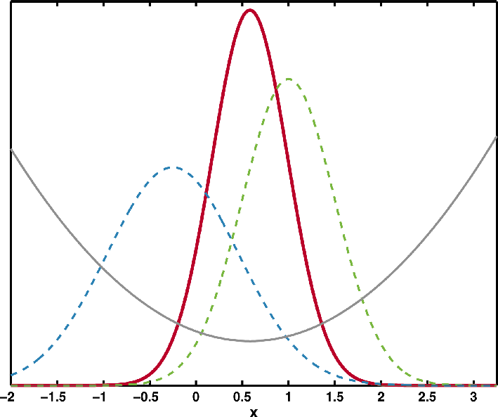
Figure 2: Data assimilation for scalar variable x assuming Gaussian error statistics. Prior estimate, given by the dashed blue line, has mean -0.25 and variance 0.5. Observation y, given by the dashed green line, has mean 1.0 and variance 0.25. The analysis, given by the thick red line, has mean 0.58 and variance 0.17. The parabolic gray curve denotes a cost function, J, which measures the misfit to both the observation and prior; it takes a minimum at the mean value of xa. From Holton and Hakim 2012.

For Gaussian distributed errors, the result for a single scalar variable (singly-dimensioned variable of one size), x, given prior estimate of the analysis value, xp, and observation y is

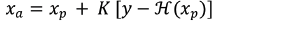(1)

where xa is the analysis value. The innovation,, represents the information from the observation that differs from the prior estimate. This comparison requires a “conversion” of the prior to the observation, which is accomplished by . For example, in a paleoclimate application,may estimate tree-ring width derived temperature data from a climate model (Fig. 1).

The weight applied to the innovation is determined by the Kalman gain, K,

(2)

where cov represents a covariance. The error variances associated with the observation and the prior estimate of the observation are given by σp and σy, respectively. Equation (1) represents a linear regression of the prior on the innovation (the denominator of K is the innovation variance). Equivalently, the Kalman gain weights the innovation against the prior, resulting in an analysis probability density function with less variance, and higher density, than either the observation or the prior (Fig. 2, red solid line, dashed green line and dashed blue line respectively). Generalizing (1) and (2) to more than one variable is straightforward, with scalars becoming vectors and variances becoming covariance matrices (for details see Brönnimann et al., this issue). These covariance matrices provide the information that spreads the innovation in space and to all variables through a Kalman gain matrix.

Application of data assimilation to the paleoclimate reconstruction problem involves determining the state of the climate system on the basis of sparse and noisy proxy data, and a prior estimate from a numerical model (Widmann et al. 2010). These data are weighted according to their error statistics and may also be used to calibrate parameters in a climate model (Annan et al. 2005).

Relationship to established methods

While there are similarities between the application of data assimilation to weather and paleoclimate, there are also important differences. In weather prediction, observations are assimilated every 6 hours, which is a short time period compared to the roughly 10-day predictability limit of the model. However, transient state estimation in paleoclimatology involves proxy data having timescales of years to centuries or longer, which generally exceeds the predictability of climate models, which are on the order of a decade. Consequently, relative errors in the model estimate of the proxy are usually much larger in paleoclimate applications. Hoever, data assimilation reconstruction may still be performed, at great cost savings, since the model no longer requires integration and each assimilation time may be considered independently (Bhend et al. 2012).

Paleoclimate data assimilation attempts to improve upon climate field reconstructions that use purely statistical methods. One well-known statistical approach for climate field reconstruction (Mann et al. 1998; Mann et al. 2008) involves limiting field variability to a small set of spatial patterns that are related to proxy data during a calibration period. Data assimilation, on the other hand, retains the spatial correlations for locations near proxies, which may be lost in a small set of spatial patterns, and also spreads information from observations in time through the dynamics of the climate model. Another distinction between data assimilation and field reconstruction approaches concerns the observation operator, , which often involves biological quantities of proxy data that have uncertain relationships to climate. Statistical reconstructions directly relate proxy data to the set of spatial patterns, which is essentially an empirical estimate of the inverse of , and therefore subject to similar uncertainty.

Current and future directions

Research on paleoclimate data assimilation is rapidly developing in many areas. For climate state estimates, a wide range of methods are currently under exploration (see Brönnimann et al., this issue), including nudging climate models to large-scale patterns derived from proxy data (Widmann et al. 2010), and variational (Gebhardt et al. 2008) and ensemble approaches (Bhend et al. 2012). Ensemble approaches involve many realizations of climate model simulations, each of which is weighted according to their match to the proxy data, either in the selection of members (Goosse et al. 2006) or through a linear combination.

Among the important obstacles to progress in paleoclimate data assimilation, some challenges are generic, such as improving the chronological dating quality of proxy records and reducing the uncertainties of the paleoclimate data. Other problems are more specific to data assimilation, such as the development of proxy forward models. Moreover, proxy data typically represent a time average, in contrast to instantaneous weather observations, although solutions that involve assimilating time averages have been proposed to tackle this problem (Dirren and Hakim 2005; Huntley and Hakim 2010). Model bias is also problematic for paleoclimate data assimilation, especially for regions with spatially sparse proxy data.

While the field of paleoclimate data assimilation is still in its infancy, these challenges are all under active research. Merging climate models and proxy data has a bright future in paleoclimate research (e.g. the P2C2 program of the U.S. National Science Foundation), and it is likely that paleoclimate data assimilation will play a central role in this endeavor.

affiliations

1Department of Atmospheric Sciences, University of Washington, Seattle, USA; ghakimuw.edu

2Research Institute for Global Change, JAMSTEC, Yokohama Institute for Earth Sciences, Japan

3Institute of Geography and Oeschger Centre for Climate Change Research, University of Bern, Switzerland

4Earth and Life Institute and Georges Lemaître Centre for Earth and Climate Research, Université catholique de Louvain, Belgium

5Department of Geographical Sciences, University of Bristol, UK

6MARUM and Department of Geosciences, University of Bremen, Germany

7KNMI, De Bilt, The Netherlands

8School of Geography, Earth and Environmental Sciences, University of Birmingham, UK

selected references

Full reference list online under: pastglobalchanges.org/products/newsletters/ref2013_2.pdf

Annan J, Hargreaves J, Edwards N, Marsh R (2005) Ocean Modelling 8(1): 135-154

Bhend J et al. (2012) Climate of the Past 8: 963-976

Goosse H et al. (2006) Climate Dynamics 27: 165-184

Widmann M et al. (2010) Climate of the Past 6: 627-644

Wikle CK, Berliner ML (2007) Physica-D 230: 1-16

Stefan Brönnimann1, J. Franke1, P. Breitenmoser1, G. Hakim2, H. Goosse3, M. Widmann4, M. Crucifix3, G. Gebbie5, J. Annan6 and G. van der Schrier7

Reliable estimations of past climate states are the foundations of paleoclimatology. Traditionally, statistical reconstruction techniques have been used, but recent developments bring data assimilation techniques to the doorstep of paleoclimatology. Here we give a short overview of transient atmospheric state estimation in paleoclimatology using data assimilation. An introduction to data assimilation as well as applications for equilibrium state estimation and parameter estimation are given in the companion papers to this special section (see also Wunsch and Heimbach 2013).

Figure 1: Schematic overview of assimilation approaches. Arrows denote steps in the procedure.

Data assimilation combines information from observations with numerical models to obtain a physically consistent estimate (termed “analysis”) of the climate state. It has been hugely successful in generating three-dimensional atmospheric data sets of the past few decades. The “Twentieth Century Reanalysis Project” (Compo et al. 2011) extended the approach as far back as 1871, but there is a limit to further extension, because conventional data assimilation relies on the availability of state observations. Paleoclimate proxies do not capture atmospheric states, but time-integrated functions of states, such as averages, in the simplest case. Therefore, for assimilating proxies, other methods are required than those applied in atmospheric sciences. We briefly present below, three groups of assimilation methods for transient atmospheric state estimation in paleoclimatology: “Classical” covariance-based approaches such as the Kalman Filter or variational techniques; approaches based on analogues such as Particle Filters; and nudging techniques. A schematic view of these methods is given in Figure 1. Note that other methods may be used for the ocean (see Gebbie 2012).

Covariance-based approaches

The assimilation problem can be formulated as a cost function J, assuming Gaussian probability distributions:

J(x) = (x-xb)T B-1 (x-xb) + (y-H[x])T R-1 (y-H[x])    (1)

where x is the analysis, xb is a model forecast, y are the observations (or proxies), H is the observation operator that mimics the observation (or proxy) in the model space, B is the background error covariance matrix and R is the observation error covariance matrix (often assumed to be diagonal). The solution to (1) in the classical Kalman form is:

x = xb + BHT(R+HBHT)-1 (y-Hxb)    (2)

where H is the Jacobian of H. Variational approaches can be used to approximate the solution. In the Ensemble Kalman Filter (EnKF), B can be estimated from the ensemble, and each member is updated individually. Normally x is a state vector. However, Dirren and Hakim (2005) have successfully extended the concept to time averages.

Data assimilation entails that x serves as an initial condition for the next forecast step. Focusing on the seasonal scale, Bhend et al. (2012) use the EnKF without updating the initial conditions (termed EKF here), which are no longer important on this scale (rather, predictability comes from the boundary conditions, including sea-surface temperatures). This conveniently allows one to use pre-computed simulations. Because x does not serve as new initial condition, it can be small and can be a vector of averaged model states (e.g. all monthly averages of a season for three variables). H can be a simple proxy forward model, i.e. a time-integrated function of elements of x.

Covariance-based approaches are powerful but computationally intensive and can be sensitive to assumptions (e.g. of Gaussian distributions), to the treatment of covariance matrices, or to the behavior of the observation operator.

Analogue approaches

Reverting to cost function (1), we can also look for an existing x, e.g. by choosing among different ensemble members. The cost function (1) reduces to:

J(x) = (y-H[x])T R-1 (y-H[x])     (3)

for x ϵ {x1, x2,...,xn}

New ensemble members are then generated for the next time step by adding small perturbations to x and the final analysis is a continuous simulation. The Particle Filter (PF, Goosse et al. 2010) approach uses a distribution of x to calculate a weighted sum of cost function contributions to (3).

In the Proxy Surrogate Reconstruction approach (PSR, Franke et al. 2011) and the Best Ensemble Member approach (BEM, Breitenmoser et al., in preparation) pre-computed simulations are used with {x1, x2,...,xn} denoting different slices of a long simulation for PSR or in the case of BEM, the same slice in an ensemble of simulations. The “analysis” in both cases is a sequence of short, discontinuous simulations. In contrast to EnKF, H may be non-differentiable (e.g. H can be a complex forward model driven by the full simulation output). R may be non-diagonal, and x may be very large (e.g. six-hourly model output over a 6 month period). However, to reconstruct the state of systems including a large number of degrees of freedom, these approaches require a huge pool of possible analogues (Annan and Hargreaves 2012).

Nudging approaches

Nudging approaches (Widmann et al. 2010) do not explicitly minimize a cost function. The distance between model state and observations is reduced by adding tendencies to (a subspace of) the model state at each time step, similar to an additional source term in the tendency equations. Following our notation:

x = xb + G (F[y] - x)    (4)

where F[y] represents the target field (derived using up-scaling method F from observations or proxies y) in the dimension of the model (sub-)space. G is a relaxation parameter.

The Forcing Singular Vectors method (van der Schrier and Barkmeijer 2005) manipulates the tendency equations as well, but adds a perturbation, which modifies the model atmosphere in the direction of the target pattern only.

Examples

Figure 2: Northern hemisphere temperature anomalies for April to September 1810 (relative to 1801-1830) from the unconstrained ensemble mean, the EKF ensemble mean, BEM (member 01), and the EKF analysis for the BEM member. Circles indicate locations and anomalies of the assimilated instrumental measurements; red squares the locations of tree-ring proxies.

Figure 2 shows April-to-September averages of surface air temperature obtained from two assimilations approaches (EKF and BEM) for the year 1810 relative to the 1801-1830 mean. Both approaches are based on the same ensemble of simulations described in Bhend et al. (2012). The ensemble consists of 30 simulations performed with ECHAM5.4 at a resolution of T63/L31 (ca. 2° x 2°), with sea-surface temperatures and external forcings as boundary conditions.

The unconstrained ensemble mean (Fig. 2 top) shows the effect of boundary conditions, here resulting in cooler than average summer temperatures following the large, but not yet localized volcanic eruption in 1809. Anomalies are small and smooth which is typical for an ensemble mean. The EKF analysis was constrained by historical instrumental observations using Eq. (2). The EKF ensemble mean suggests a more pronounced cooling over northern Europe, but over most regions (due to lack of observations) it is close to the unconstrained ensemble mean. BEM was constrained with tree rings from 35 locations. The VS-lite tree growth model (Tolwinski-Ward et al. 2011) was used as H and Eq. (3) was minimized. BEM identifies member 01 as the best fitting one. This member exhibits large anomalies in Alaska and Eurasia, but due to the small ensemble size little regional skill is expected (Annan and Hargreaves 2012). For instance, it does not fit well with instrumental observations over Europe. The same member in the EKF analysis (Fig. 2, bottom) shows a better correspondence, but we loose the advantage of having the full 6-hourly model output available.

Limitations and future directions

Paleoclimatological applications are much more disparate than atmospheric sciences in terms of time, time scales, systems analyzed, and proxies used. Therefore, a plurality of data assimilation approaches is a logical way forward. However, all approaches still suffer from problems and uncertainties. Ensemble approaches (PF, EnKF, EKF) provide some information on the methodological spread, which however represents only one (difficult to characterize) part of the whole uncertainty. Further uncertainties are related to model biases, limited ensemble size, errors in the forcings and proxy data. Validation of the approaches using pseudo proxies in toy models and climate models and validation of the results using independent proxies is therefore particularly important. Any approach, however, fundamentally relies on a good understanding of the proxies.

affiliations

1Institute of Geography and Oeschger Centre for Climate Change Research, University of Bern, Switzerland; stefan.broennimanngiub.unibe.ch

2Department of Atmospheric Sciences, University of Washington, Seattle, USA

3Earth and Life Institute and Georges Lemaître Centre for Earth and Climate Research, Université catholique de Louvain, Belgium

4School of Geography, Earth and Environmental Sciences, University of Birmingham, UK

5Department of Physical Oceanography, Woods Hole Oceanographic Institution, USA

6Research Institute for Global Change, JAMSTEC, Yokohama Institute for Earth Sciences, Japan

7KNMI, De Bilt, The Netherlands

selected references

Full reference list online under: pastglobalchanges.org/products/newsletters/ref2013_2.pdf

Bhend J et al. (2012) Climate of the Past 8: 963-976

Dirren S, Hakim GJ (2005) Geophysical Research Letters 32, doi:10.1029/2004GL021444

Goosse H (2010) Journal of Geophysical Research 115, doi:10.1029/2009JD012737

van der Schrier G, Barkmeijer J (2005) Climate Dynymics 24: 355-371

Widmann M et al. (2010) Climate of the Past 6: 627-644

Tamsin L. Edwards1, J. Annan2, M. Crucifix3, G. Gebbie4 and A. Paul5

We introduce data assimilation methods for estimating past equilibrium states of the climate and environment. The approach combines paleodata with physically-based models to exploit their strengths, giving physically consistent reconstructions with robust, and in many cases, reduced uncertainty estimates.

Those seeking to understand the Earth’s past usually take one of two approaches: reconstructing paleoclimate and paleo-environmental states from proxy data derived from natural archives such as ice cores and trees; or simulating them with earth system models that contain theoretical knowledge of physical processes.

Proxy-based reconstructions are based on observations of the real world, but most consider data points independently rather than accounting for correlations in space, time and between climate variables. Therefore they risk being physically inconsistent. Models incorporate aspects of physical consistency, but are imperfect and are tested during development only with present day observations.

Data assimilation produces “best-of-both-worlds” estimates that combine observational and theoretical information while not ignoring their limitations. We discuss data assimilation for estimating past equilibrium states of the earth system such as climate and vegetation. We use the term “paleodata” for measurement-based data: either the observations of proxies or the statistical reconstructions derived from them.

Aims and methods

Equilibrium state, or “time slice”, data assimilation is estimation of a snapshot in time during which it is assumed the state variables are not changing. The state estimates may be the primary scientific aim or simply a “bonus” of calibrating model parameters (Annan et al., this issue).

Time slice estimation is a natural starting point in data assimilation because it is more straightforward than estimating a transient state (Brönnimann et al., this issue) and is particularly appropriate if spatial patterns are more important than temporal changes or if the model is computationally expensive. For a given computational resource time slice estimation permits more complete exploration of model uncertainties in parameters, structure, and inputs. Another advantage of a focus on time slices is that for eras studied by the Paleoclimate Model Intercomparison Project (PMIP) relatively large quantities of paleodata and simulations are available. Most data assimilation estimates of equilibrium paleo-states are therefore of the Last Glacial Maximum (LGM: 21 ka cal BP), the most recent era for which annual mean climate is substantially different to the present that also has a long history of study by PMIP.

We use model simulations in paleo-state estimation because models provide links across different locations, times (relevant to transient or multi-state estimation) and state variables. This has two advantages: it helps ensure the resulting state is physically consistent, and it also means we are not limited to assimilating the same variables we wish to estimate. We could assimilate data in one place to estimate another, or assimilate temperature data to estimate precipitation, or assimilate variables corresponding to the outputs of a model to estimate variables corresponding to the inputs. The last are termed “inversion” methods, such as estimating atmospheric variables or terrestrial carbon from paleo-vegetation records (e.g. Guiot et al. 2000; Wu et al. 2007; Wu et al. 2009; Pound et al. 2011) or estimating oceanic variables from paleo-tracer records (e.g. LeGrand and Wunsch 1995; Roche et al. 2004).

Data assimilation requires the following ingredients: paleodata with uncertainty estimates, simulations with uncertainty estimates, and a metric to quantify the dissimilarity, or “distance”, between the two. Climate state estimates are obtained by searching for the simulation(s) closest to the paleodata (“optimization”) or calculating a weighted combination of the two (“updating”).

Distance is usually measured with the standard metric for normally distributed model-data differences, i.e. the sum of squared differences weighted by the uncertainties, though some use ad-hoc or fuzzy metrics (e.g. Guiot et al. 2000; Wu et al. 2007; Gregoire et al. 2010). For non-continuous variables, for example with a threshold, variables must be transformed or a non-Gaussian metric chosen (e.g. Stone et al. 2013).

Optimisation methods search for the simulation with the minimum distance from paleodata. One approach uses numerical differentiation of the model with respect to the parameters, essentially least-squares fitting of a line or curve to one-dimensional data (e.g. LeGrand and Wunsch 1995; Gebbie and Huybers 2006; Marchal and Curry 2008; Burke et al. 2011; Huybers et al. 2007; Paul and Losch 2012). Another approach generates an ensemble of simulations using many different parameter values and then selects the members with the smallest model-data distance (“perturbed parameter ensemble” methods; e.g. Gregoire et al. 2010).

Updating methods combine model and paleodata estimates. Typically the model estimates are generated with a perturbed parameter ensemble, which permits well-defined sampling of parameter uncertainties; the model estimates are reweighted with the model-data distance using Bayesian updating (e.g. Guiot et al. 2000; Wu et al. 2007; Wu et al. 2009; Holden et al. 2009; Schmittner et al. 2011).

Interpretation

Figure 1: LGM annual mean temperature anomalies from: (A) surface air temperature (SAT) reconstructions based on pollen and plant macrofossils (Bartlein et al. 2010); (B) sea surface temperature (SST) reconstructions based on multiple ocean proxies (MARGO et al. 2009); (C, D) simulations from the HadCM3 general circulation model (mean of 17 member perturbed parameter ensemble; Edwards, unpublished data). Data assimilation estimates generated by updating with SAT reconstructions (E, F), and both SAT and SST reconstructions (G, H). Gray areas indicate regions with low signal-to-noise: magnitude of temperature anomaly is less than 3σ of uncertainty estimates.

Figure 1 illustrates some strengths of data assimilation. The model propagates information from LGM surface air temperature (SAT) reconstructions over land to other regions, and to sea surface temperatures (SST). In this example assimilating SAT reconstructions produces an SST estimate with a warming at the LGM in the northern North Atlantic, which is consistent with the SST reconstructions. Uncertainties are reduced relative to the model estimate in most locations (grayed out areas are reduced).

How should we interpret assimilated paleo-states? Optimization methods select a single best simulation so the state estimate is physically self-consistent according to the model. But the state estimate from updating methods is a combination of multiple model simulations and paleodata, therefore interpretation requires more care. An ensemble mean anomaly of zero might correspond to a wide spread of positive and negative results; this would be reflected in large model uncertainties. A spatially coherent signal with small uncertainty might emerge from an ensemble after assimilating a single “pinning point” from paleodata; this signal should be physically consistent because it arises from the model physics. Such considerations are common to all multi-model ensemble summaries and reanalyses.

For statistically meaningful results it is essential to use a distance metric grounded in probability theory, i.e. corresponding to a particular distribution of model-data differences (“likelihood function” in Bayesian terms). This might preclude the use of non-standard variables such as biomes.

Data assimilation is a statistical modeling technique and should be evaluated. Testing the method with pseudo-paleodata can help avoid the (literal) pitfalls of finding local rather than global minima in high-dimensional spaces.

Future directions

Data assimilation is a formal method that not only highlights model-data discrepancies but also corrects them. It can be challenging, because it requires a process-based model and reliable estimation of uncertainties for both paleodata and simulations.

For paleodata, difficulties may arise from dating and time averaging. But improvements in estimating reconstruction uncertainties can be made by using forward modeling approaches (e.g. Tingley et al. 2012). These approaches allow greater freedom in specifying the behavior of climate-proxy relationships (such as nonlinearity and multi-modal uncertainties) and enables uncertainties to cascade through the causal chain to allow full probabilistic quantification of the unknown state. Using physically -based forward models for reconstruction, i.e. data assimilation, incorporates information about the relationships between locations, times and variables and therefore minimizes the risk of physical implausibility. The long-term goal may be forward physical modeling of the whole causal chain from radiative forcings to proxy archives (e.g. Roche et al. 2004; Stone et al. 2013).

For paleo-simulations, we do not need models to be complex or state-of-the-art, but we do need to estimate their uncertainties. If they are complex it is difficult to generate their derivatives with respect to the parameters. If they are expensive it is difficult to sample, and therefore to assess, their uncertainties. Thoughtful experimental design with statisticians, and perhaps also statistical modeling of the physical model (known as “emulation”; e.g. Schmittner et al. 2011), can help in this regard. A research priority is to estimate the discrepancy between a model and reality at its best parameter values, and how this varies across different eras. New updating methods are emerging that use the PMIP multi-model ensemble to explore structural uncertainties. For example, Annan and Hargreaves (2013) use the linear combination of ensemble members that best matches the paleodata.

These challenges are worth tackling for the substantial benefits. Information from paleodata can be extrapolated to other locations, times and state variables, and uncertainties are smaller (or at worst, the same) than those of the individual model or proxy-based estimates.

affiliations

1Department of Geographical Sciences, University of Bristol, UK; tamsin.edwardsbristol.ac.uk

2Research Institute for Global Change, JAMSTEC, Yokohama Institute for Earth Sciences, Japan

3Earth and Life Institute and Georges Lemaître Centre for Earth and Climate Research, Université catholique de Louvain, Belgium

4Department of Physical Oceanography, Woods Hole Oceanographic Institution, USA

5MARUM - Center for Marine Environmental Sciences and Department of Geosciences, University of Bremen, Germany

selected references

Full reference list online under: pastglobalchanges.org/products/newsletters/ref2013_2.pdf

Bartlein P et al. (2010) Climate Dynamics 37(3-4): 775-802

Guiot J et al. (2000) Ecological Modelling 127(2-3): 119-140

Schmittner A et al. (2011) Science 334: 1385-1388

MARGO Project Members (2009) Nature Geoscience 2: 127-132

Stone EJ, Lunt DJ, Annan JD, Hargreaves JC (2013) Climate of the Past 9: 621-639