PAGES Magazine articles
Keely Mills1, S. McGowan2, É. Saulnier-Talbot3 and P. Gell4
Kuala Lumpur, Malaysia, 15-17 February 2017
The first two meetings of the Aquatic Transitions working group, whilst focused on a global agenda, were dominated by members from Europe and North America. Early screening of metadata available from these members highlighted major data gaps in China, South America, Africa, and Tropical Asia. To address some of these gaps, Aquatic Transitions "piggy-backed" on a number of international conferences in China (International Paleolimnology Symposium, Lanzhou, August 2015; INTECOL Wetlands Conference, Changshu, September 2016) to raise our profile and recruit potential members from Asia. This third meeting focused efforts in SE Asia, and welcomed 30 participants (20 from Tropical Asia) to Kuala Lumpur. The group comprised six Aquatic Transitions "veterans", eight established academics with expertise in the region, eight early-career researchers, seven MSc and PhD students, and a stakeholder from the Forestry Research Institute of Malaysia.
 |
|
Figure 1: During the workshop, we compiled a list of published paleolimnological research from across the south east Asia region. We are now in the process of synthesizing this data into a paper titled "Paleoenvironmental change from SE Asian lacustrine sites". |
Given the new group composition, day one began with introductions to PAGES and Aquatic Transitions, and to what we thought we knew about lake systems in the tropical Asia region, summarizing previously published work (Fig. 1). All participants gave "speed talks", introducing themselves, their research, and the lake systems on which they worked. The afternoon closed with a short lecture on "what is paleolimnology" for those who were less familiar with its use and application.
On the second day, participants rotated between six discussion groups focused on the key topics: SE Asia regional review; Ecosystem services; Linking lakes and drivers; Paleo-problem solving; Lakes as socio-ecological systems; and Freshwater biodiversity. In the afternoon, participants were updated on outputs from the previous Aquatic Transitions meetings (with a focus on populating the UCL-hosted LakeCores database), published papers and those in preparation, and a "Developments in Paleoenvironmental Research" volume that was solicited by Springer. During this session, a number of abstracts were prepared as part of the book proposal – with contributions from early-career members. As part of the database activities, data and publications from the Tropical Asia region were compiled during the meeting (Fig. 1). The day ended with a public lecture hosted by University of Nottingham’s Malaysia Campus as part of the Mindset Research Centre lecture series. Three short lectures were delivered by Keely Mills, Nathalie Dubois and Suzanne McGowan under the title "Understanding the Anthropocene using lake sediment records". The talk attracted over 80 attendees and is available as a podcast here: http://mindset.my/content/talk021.html
The final day focused on stakeholders and regional engagement and capacity building. As Aquatic Transitions moves forward, and in an attempt to have our outputs utilized outside academia, it is important to identify key stakeholders. Small groups mapped stakeholder groups, categorizing those who have a high level of interest in our work, and those who have a high level of influence. This was a productive exercise to think more broadly about our interactions when designing research projects for impact. The meeting concluded with discussions on the next steps for Aquatic Transitions – the initial three-year phase ends in December 2017. Community interest was gauged to assess whether we should apply for a second phase to allow us to include more researchers from regions that lack data. Attendees at the Tropical Asia workshop provided excellent support, and it has been agreed that whilst we tie up Phase 1 loose ends, we submit an application in early 2018 for Phase 2. Future workshops in Africa and South America would boost interest and encourage global participation. Finally, regional leaders to help drive Phase 2 forward were identified.
affiliations
1British Geological Survey, Keyworth, UK
2School of Geography, University of Nottingham, UK
3Université Laval, Québec, Canada
4Water Research Network, Federation University Australia, Ballarat, Australia
contact
Keely Mills: kmil bgs.ac.uk
Nikita Kaushal1 and Laia Comas-Bru2
Second SISAL meeting, Stockholm, Sweden, 20-22 September 2017
PAGES’ SISAL (Speleothem Isotope Synthesis and Analysis) working group is creating a systematic global synthesis of speleothem isotopic records (Comas Bru et al. 2017a). Beyond the creation of the database, SISAL also aims to understand and showcase how speleothem data can be used in paleoclimate modeling studies. Data synthesis combined with suitable modeling targets can help reduce uncertainty and improve interpretations in both. Such data-model comparisons can also help refine our quantitative understanding of past climate events and enhance credibility of model projections (Schmidt 2010). At the time of this workshop, we had 208 of ~577 speleothem-based climate records in the database with more records being added every week (see Fig. 1 in Comas Bru et al. 2017b for a global map with identified records). The first version of the SISAL database will be released in early 2018.
Seventeen SISAL members (including eight early-career researchers and six researchers from the PMIP modeling community) met to discuss isotope-enabled model evaluations using the database and how the SISAL database should be made available to end-users such as the paleoclimate modeling community. The meeting took place at the Navarino Environmental Observatory in Stockholm, Sweden, and was organized by a group of SISAL members from different universities. On Day 1, participants presented research on prospects for speleothem-model evaluations targeting specific climate questions, periods and regions. Presentations were also given by stakeholders such as IsoNet (Isotopes for Tropical Ecosystem Studies) and the proxy data synthesis working group of PalMod (www.palmod.de). This was followed by a discussion on the best-practice methods to quantify uncertainties on the age and isotope measurements in SISAL and the most convenient way for modelers to understand and incorporate these uncertainties when using the database. There were subsequent discussion sessions on proof-of-concept exercises using SISAL and existing isotope-enabled simulations. These discussions were formalized through breakout sessions, where tasks were delegated to SISAL members. Throughout the day, we identified gaps in data coverage for key time periods in specific regions.
 |
|
Figure 1: Time coverage of the records (n=208) in SISAL_v0 (September 2017) for different regions: Europe (36-75°N, 30°W-30°E), Middle East and Africa (45°S-36°N, 30°W-60°E), Asia (10-60°N, 60-130°E), Oceania (10-60°S, 90-180°E), North and Central America (10-60°N, 50-150°W) and South America (60°S-10°N, 30-150°W). |
Day 2 kicked-off designing the contents of the SISAL presentation for the PMIP4 meeting the following week to showcase the major features of the interim SISAL database (Fig. 1). This was followed by a discussion on how to address key questions related to the climate interpretation of speleothem isotopic data using paleoclimate model outputs. Lastly, there were hands-on sessions centered on advancing the first publications emerging from the SISAL database. Sections of the paper describing the database were jointly written by SISAL members in multiple breakout sessions and further papers focusing on specific climate questions were outlined. These outlines will be shared with the wider SISAL community to give it the opportunity to participate in the projects. Day 2 also saw a short presentation on the PAGES working group DAPS (Paleoclimate Reanalyses, Data Assimilation and Proxy System Modelling) to identify possible synergies to emerge from a SISAL-DAPS collaboration. We decided to organize short meetings with both groups at widely attended, large geoscience conferences in 2018 to promote further discussions. Day 3 brought the workshop to a close with a recap discussion on our next steps towards SISAL’s third meeting in October 2018 and developing a timeline for the working group’s future activities.
SISAL encourages ideas for big data analyses that can be achieved with this new dataset. For more information about SISAL or how to get involved, go to pastglobalchanges.org/sisal
acknowledgements
We thank PAGES, the University of Reading, University College Dublin, Navarino Environmental Observatory in Stockholm University, Savillex and John Cantle for their financial support.
affiliations
1Department of Earth Sciences, University of Oxford, UK
2School of Earth Sciences, University College Dublin, Ireland
contact
Nikita Kaushal: nikitageologistgmail.com
references
Comas Bru L et al. (2017a) PAGES Mag 25: 129
Laia Comas-Bru1, Y. Burstyn2,3 and N. Scroxton4
First SISAL meeting, Dublin, Ireland, 21-23 June 2017
 |
|
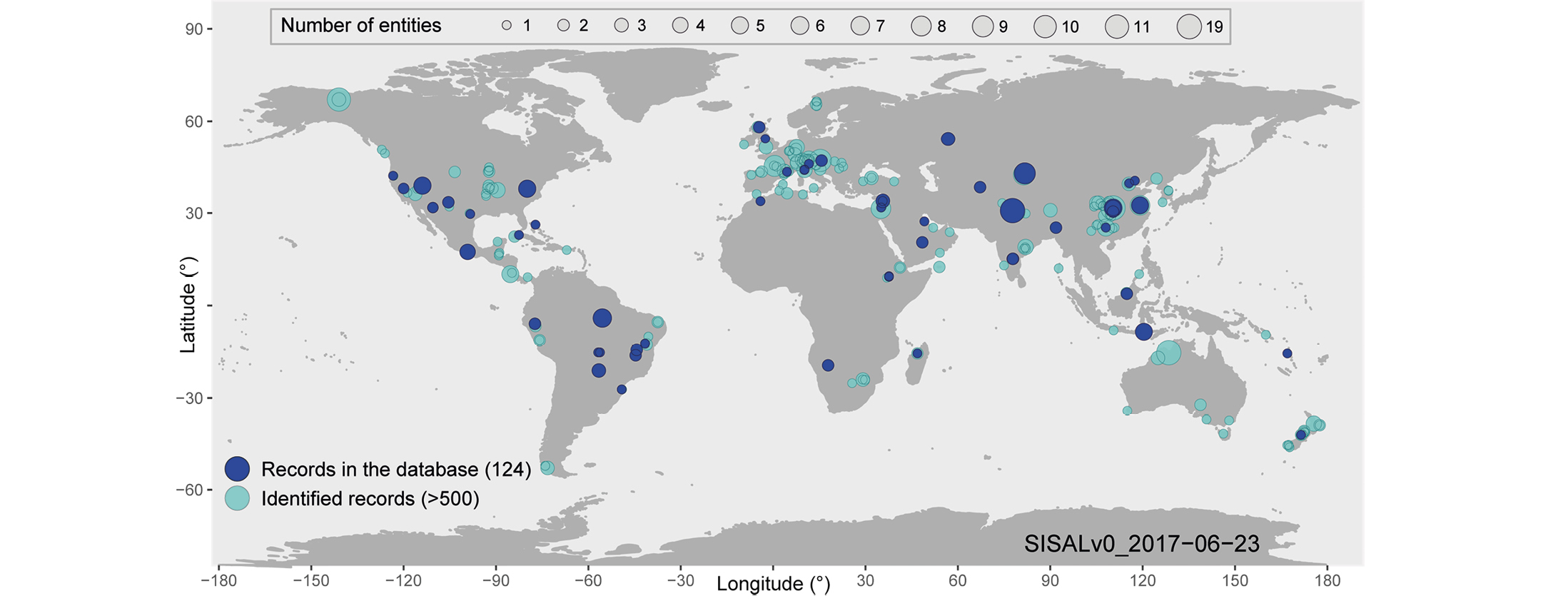
Figure 1: Global map showing the records uploaded to SISAL’s database (n=124; dark blue) at the end of the workshop versus the 500+ records identified by SISAL members (cyan). |
Speleothem based paleoclimate records have risen in prominence over the last few years as long-term, precisely dated, continental archives of past changes in the hydrological cycle. But these valuable records have yet to make significant contributions to recent big data syntheses. For example, only seven records are included in the standard Palaeoclimate Modelling Intercomparison Project (PMIP) benchmark dataset (Harrison et al. 2014). A synthesis of existing speleothems records has great potential for exploring regional and global-scale past changes in the hydrological cycle, as well as for evaluating the ability of climate models that explicitly simulate water and carbon isotopes to capture hydroclimate variability through data-model comparisons. To address these issues and to increase the impact of speleothem research in general, PAGES’ SISAL (Speleothem Isotopes Synthesis and Analysis) working group is creating a systematic global synthesis of speleothem δ18O and δ13C records (Fig. 1 and Comas Bru et al. 2017).
Twenty-three SISAL members (including 12 early-career researchers) met for the first SISAL workshop. The meeting took place at the UCD O’Brien Centre for Science at University College Dublin, Ireland, and was coordinated by Laia Comas Bru (University College Dublin, Ireland) and Sandy Harrison (University of Reading, UK). Over three days, workshop participants established the framework for the SISAL database, discussed potential data analysis projects and added entries to the database. On Day 1, speleothem scientists representing all continents (apart from Antarctica) presented reviews of speleothem research and existing records in their regions, and climate and karst/speleothem modelers also introduced how the SISAL database could be used by their communities. These presentations were followed by an interactive introduction to the preliminary structure of the database that was prepared in advance of the meeting by SISAL steering committee members. During this working session led by Kamolphat Atsawawaranunt (University of Reading, UK), participants had the opportunity to test the structure and contents of the database by entering individual data sets and raising any questions or issues. Based on this feedback, Day 2 was dedicated to group discussions where workshop participants deliberated issues such as identifying the essential metadata needed for SISAL’s purpose, dealing with ambiguous terminology and ensuring that the database includes the key parameters and information required for assessing age models. Further discussions on data collection strategy and forward planning of analyses served to shape the key points for the group’s first scientific papers. Day 3 brought the workshop to a close with a recap discussion on the next steps before SISAL’s second meeting in September 2017 (Kaushal and Comas Bru 2017) and developing a timeline for the working group’s activities.
One important decision made during this three-day workshop was the nomination of "regional coordinators", who will liaise with authors publishing on speleothems from a given region and will be responsible for the initial quality control of records. We are confident this approach will enormously help facilitate data entry and also involve a wider group of scientists in the SISAL project, ensuring its success. A complete list of regional coordinators is available on our webpage.
SISAL welcomes paleoscientists interested in the curation of the database and encourages ideas for big data analyses that can be achieved with this new dataset. Those researchers with data to add to the database are encouraged to contact the regional coordinator for the geographic area of their stalagmite record. The first version of the database closes 31 December 2017. For more information about SISAL and how to get involved, go to pastglobalchanges.org/sisal
acknowledgements
We would like to thank PAGES, European Geosciences Union (EGU), iCRAG (Irish Centre for Research in Applied Geosciences), Geological Survey Ireland, Quaternary Research Association UK and the University of Reading for their financial support.
affiliations
1School of Earth Sciences, University College Dublin, Ireland
2Geological Survey of Israel, Jerusalem, Israel
3Hebrew University of Jerusalem, Israel
4Department of Geosciences, University of Massachusetts Amherst, USA
contact
Laia Comas Bru: laia.comasbruucd.ie
references
Comas Bru L et al. (2017) PAGES Mag 25: 129
Thomas B. Chalk1, E. Capron2,3, M. Drew4 and K. Panagiotopoulos5
Molyvos, Greece, 28-30 August 2017
 |
|
Figure 1: (A) 65°N summer solstice insolation, (B) Atmospheric CO2 concentration, Allan Hills vertical error bars indicate 2σ spread with horizontal age uncertainty, (C) Global LR04 benthic stacked δ18O (blue), ODP1123 seawater δ18O (black). The MPT and the "typical 41 ka-world" intervals are highlighted in grey and yellow respectively. |
A defining feature of the Quaternary is the quasi-periodic expansion and contraction of major Northern Hemisphere ice sheets. Before ~1.25 million years ago (Ma), glacial-interglacial cycles appear symmetric with smaller ice volumes and a period of 41 thousand years (ka, Fig. 1). Between ~1.25 to 0.7 Ma, the Earth’s climate underwent a fundamental change, the Mid-Pleistocene Transition (MPT), where the dominant frequency of climate cycles changed from 41 to 100 ka. A full understanding of these modes of variation and the cause of such a change occurring under a relatively similar orbital forcing is still missing. To advance this topic, the third QUaternary InterGlacialS (QUIGS) workshop gathered 29 delegates to review the current science of the 41 ka-world interglacials and the underlying causes of the MPT. The outcome combines information from paleoclimatic archives together with insights from ice-sheet and climate modeling, producing future research directions.
Interglacials of the 41 ka world
Based on published and emerging paleoclimatic records extending beyond the MPT, similarities and differences in 100 ka-world (post-MPT) interglacials were identified. In brief, the 41 ka-world (pre-MPT) interglacials are generally more symmetrical in benthic δ18O records than post-MPT interglacials (Fig. 1). Interglacial values are similar but the duration of pre-MPT glacial terminations and inceptions can differ. The high latitudes are characterized by warmer oceanic and continental surface conditions during pre-MPT interglacials. While pre- and post-MPT glacial atmospheric CO2 levels differ, boron isotope-based reconstructions suggest similar interglacial levels (Fig. 1). The relatively high pre-MPT glacial-interglacial CO2 and sea-level variability is not yet simulated in modeling studies. Pre-MPT interglacials are characterized by a millennial-scale climatic variability but the presence of a bipolar seesaw mechanism at their onset, a key millennial-scale feature of the post-MPT interglacials, cannot yet be assessed.
Sea-level and ice-volume estimates, as well as most reconstructions of more regional climate and environmental patterns during pre-MPT interglacials, have large uncertainties and limited temporal resolutions.
To provide further insights on the nature of pre-MPT interglacials, we encourage future investigations to focus on generating high-resolution datasets across a time slab characterized by typical pre-MPT glacial-interglacial cycles i.e. from Marine Isotopic Stage (MIS) 42 to MIS 46. We hope also that this will generate interest within the modeling community.
The MPT and underlying causes
The MPT, referring both to the change in frequency and intensity of glacial-interglacial cycles between 1.25 and 0.7 Ma, is characterized by multiple events identified in ocean circulation intensity proxies. It is mostly considered to be either driven by (i) an atmospheric CO2 concentration decline, triggered by weathering or enhanced ocean uptake and storage or (ii) the removal by glacial erosion of thick sediment (regolith), exposing a high-friction crystalline Precambrian Shield bedrock, which increases ice stability, and an attendant change in the ice-sheet response to orbital forcing. Modeling studies have not fully reconciled the "regolith" hypothesis and questions remain over the timing of the regolith removal and the consequent ice-sheet response.
Progression on the causes of the MPT requires obtaining additional CO2 reconstructions with reduced uncertainties. Boron-derived CO2 data are coherent with direct CO2 measurements performed on 1 Ma-old ice samples (Fig. 1) but the drilling of an "Oldest Ice" core back to 1.5 Ma (Fischer et al. 2013) would offer a large increase in confidence about the evolution of the climate-carbon cycle interactions across the MPT.
An article summarizing the ideas about the MPT is being prepared. New data, modeling exercises and ideas emerging from them should appear in the next few years, and QUIGS will return to this topic during its second phase, starting in 2018.
affiliations
1Ocean and Earth Science, University of Southampton, UK
2Centre for Ice and Climate, University of Copenhagen, Denmark
3British Antarctic Survey, Cambridge, UK
4Physics and Physical Oceanography, Memorial University of Newfoundland, St John’s, Canada
5Institute of Geology and Mineralogy, University of Cologne, Germany
contact
Emilie Capron: capronnbi.ku.dk
references
Bereiter B et al. (2015) Geophys Res Lett 42: 542-549
Elderfield H et al. (2013) Science 337: 704-709
Fischer H et al. (2013) Clim Past 9: 2489-2505
Higgins JA et al. (2015) PNAS 112: 6887-6891
>Hönisch B et al. (2009) Science 324: 1551-1554
Andreas Schmittner1, G. Martínez-Méndez2, A.C. Mix1 and J. Repschläger3
Corvallis, USA, 27-29 June 2017
The last deglaciation, which is Earth's climatic transition from the Last Glacial Maximum (LGM, ~21 ka BP) to the Holocene (current interglacial period; ~10 ka BP), is still not fully understood. The associated rise in atmospheric CO2 and related changes in ocean circulation and carbon storage remain puzzling. Carbon isotopes (δ13C) are influenced by ocean circulation and carbon cycling, including the biological pump and air-sea gas exchange, and preserved in the sedimentary record in fossil shells of benthic foraminifera (unicellular organisms living at the sea floor). The PAGES working group Ocean Circulation and Carbon Cycling (OC3) aims to synthesize benthic δ13C sediment data globally to reconstruct and understand the mechanism of natural climate and carbon cycle changes with a focus on the last deglaciation.
 |
|
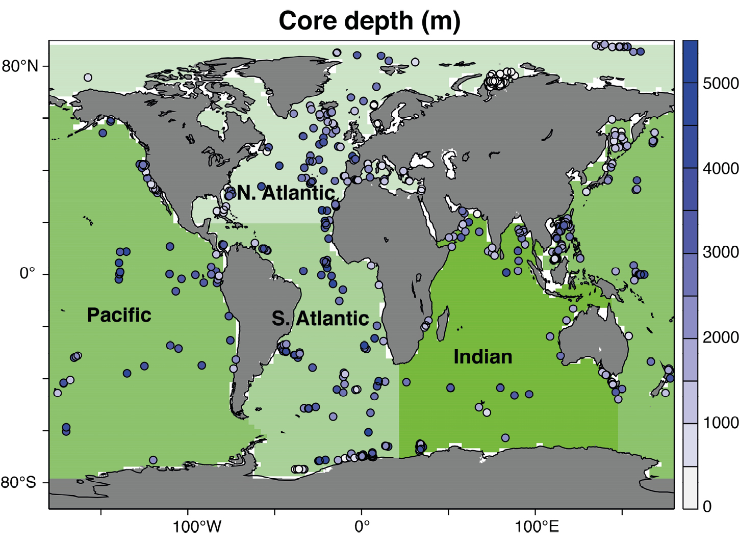
Figure 1: Map of core locations of the current OC3 down-core database. Also indicated are the regions for which different groups will perform syntheses and data quality control. |
The current, second OC3 phase focuses on down-core data syntheses in different ocean basins (Fig. 1). Goals of this second OC3 workshop were to discuss the progress and first analyses of the data collection, issues of database structure, scientific questions, and possible publications. Talks presented new modeling results on changes in meltwater fluxes during the last deglaciation, and effects of their spatial distribution on ocean circulation. Model results also explored connections between the Atlantic Meridional Overturning Circulation (AMOC), deep ocean carbon storage and isotope distributions, and atmospheric CO2. A presentation on age-model uncertainty showed differences of more than 1,000 years depending on the method used to construct the age model (radiocarbon versus oxygen-isotope alignment versus surface-property alignment). Down-core data from the North Atlantic raised the question of northern versus southern sources for reconstructed, very depleted δ13C and δ18O deep water (Repschläger et al. 2015; Keigwin and Swift 2017), whereas negative δ13C excursions in intermediate waters may be explained by changes in the efficiency of the biological pump (Lacerra et al. 2017).
Presentations on Pacific Ocean syntheses showed that the water-mass geometry in the southeast Pacific did not substantially change during the LGM and suggested larger than previously thought mean-ocean δ13C change during the deglaciation, which may challenge existing interpretations about changes in terrestrial carbon storage. A decoupling of the Pacific from the Atlantic circulation during the LGM was suggested by a comparison of δ13C depth transects from the southwest Pacific and the southwest Atlantic. The single presentation about the Indian Ocean confirmed earlier studies linking changes in AMOC with monsoonal variations during the last deglaciation. The Indian Ocean and cores from intermediate depths are currently underrepresented in OC3. Presentations on ice-core data included updates to age models and highlighted rapid and coeval changes in CH4, CO2 and δ13CCO2, not only during the last deglaciation but also for earlier parts of the last glacial cycle.
LinkedEarth (http://linked.earth; a partner project of PAGES’ 2k Network), a new, searchable, open-source, wiki-like platform for paleoclimate data compilation and curation, was introduced to the participants including a tutorial. Participants agreed to use this platform to publish the final OC3 database product.
Discussions noted differing data quality among sediment cores. Since the objective of OC3 is to include all data, it was recommended that information on data quality, including species used, age models and uncertainties, time resolution, and analytical errors, will need to be reported in the database. All data will be quality checked and flagged by multiple scientists according to their regional expertize. Initial groups for the North Atlantic, the South Atlantic, and the Pacific have already been formed. All groups are open to participation from interested colleagues.
OC3 plans to publish three regional syntheses and one global synthesis paper. The next and final OC3 meeting will be in Cambridge, UK, from 13-16 September 2018, preceded by informal meetings at the AGU Fall and Ocean Sciences meetings.
affiliations
1College of Earth, Ocean, and Atmospheric Sciences, Oregon State University, Corvallis, USA
2MARUM-Center for Marine Environmental Science, University of Bremen, Germany
3Department Climate Geochemistry, Max-Planck Institute for Chemistry, Mainz, Germany
contact
Andreas Schmittner: aschmittcoas.oregonstate.edu
references
Keigwin LD, Swift SA (2017) PNAS 114: 2831-2835
Peter Ditlevsen1 and Michel Crucifix2
Ice ages are paced by astronomical forcing, but how centennial variability affects their dynamics is still unknown.
A common explanation of ice ages asserts that they result from a chain of responses, which follow and then amplify the effects of the changes in the distribution of incoming solar radiation along the seasons and along latitudes. This is the modern interpretation of the Milankovitch theory. From this perspective, the presence of a 100-ka component dominating the frequency spectrum of proxies for ice ages has often been presented as a puzzle. True, changes in eccentricity modulate the amplitude of precession peaks at a period of about 100 ka, but the spectrum of insolation time series do not contain an amplitude peak at this period. Since the dominant period of response differs from the dominant period of forcing, the feedbacks between components of the climate system must involve some non linearity. It was then observed that the dominance of such non linear feedbacks opens the possibility that ice ages may even arise as a self-sustained cycle. With this possibility in mind, the astronomical forcing is often prudently presented as the "pacemaker" of an internal oscillation rather than a primary "driver".
The SPECMAP days
One of the objectives of the Spectral Mapping Project (SPECMAP) in the 1980s was, precisely, to investigate such dynamics (Imbrie et al. 1992). The methodology consisted of filtering climate records along frequency bands at about 1/20, 1/40 and 1/100 ka-1 in order to characterize the amplitudes of different climatic variables, and estimate leads and lags across them.
 |
|
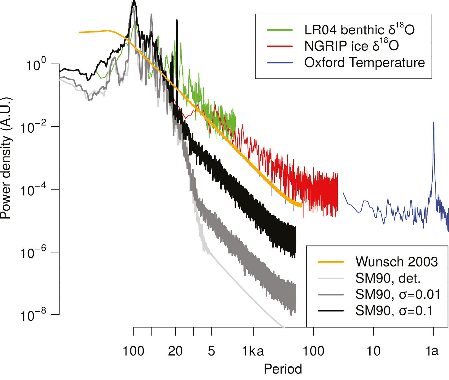
Figure 1: Periodogram of paleoclimatic records: LR04 benthic stack (green), NGRIP isotope record (red), Oxford temperature data adapted from Shao and Ditlevsen (2016; blue), compared to the spectra estimated for the Wunsch (2003) stochastic model (orange), and the Saltzmann Maash 1990 model (thick grey and black, with different levels of added noise; adapted from Crucifix et al. 2016). |
In parallel, theorists developed and studied small numerical models expressed in the form of time-difference equations representing interactions between climate components such as ice sheets and the carbon cycle. In such reduced models, the relaxation timescales, which encode the typical response time of system components, are generally of several millennia. Hence, by design, these models do not include variability at millennial frequencies, let alone centennial variability. The idea that justifies only focusing on the representation of the dynamics at a given timescale without caring much about faster dynamics is the hypothesis of timescale separation (Saltzman 1990). This is also what Lovejoy (2017) refers to as the "scale-bound view" in this issue. Unsurprisingly, thus, the power spectrum of the output of such time-difference models shows amplitude peaks at periods of ~20, 40 and 100 ka and essentially no power at shorter or longer periods (Fig. 1, the "SM90 deterministic" model).
A drunkard's walk
Early on, however, several investigators (e.g. Pisias and Moore 1981) remarked that when the power spectrum of climate variations is plotted on a log-log form, the so-called Milankovitch peaks become almost anecdotal. The visual impression is rather that of a noisy process encompassing slow and fast variability. It turns out that, from the point of view of mathematics, it is not very difficult to construct simple stochastic processes having essentially the same power spectrum as that of the paleoclimatic data. The following model was proposed by Wunsch (2003): Imagine that ice volume may randomly increase or decrease, with a statistical preference for increase (because, say, that the average conditions are colder than in the early Pliocene and favor glaciation). In the parlance of dynamical systems theory this is called a random walk with a drift, perhaps better imaged as “a drunkard's walk”. This kind of drifted random walk will unavoidably reach, sooner or later, a threshold which we fix arbitrarily, and at which point we decide that deglaciation occurs.
The two free parameters (drift and threshold) of this model can easily be adjusted to reproduce the broad characteristics of the paleoclimatic deep-ocean sediment record of ice ages. The model spectrum has no scale separation from the high frequencies down to the 100-ka cycle. Milankovitch forcing may then be parsimoniously re-injected either on the drift of the random walk or in a time varying size of the threshold (Huybers and Wunsch 2005).
Two views on ice ages
We thus face two different views on ice ages. In the first view, the modern Milankovitch theory explains ice ages as the result of multiple feedbacks which operate at the timescale of several millennia. Simple deterministic models are the expression of this view and they can be impressively successful at reproducing the broad time evolution of ice age proxies all over the Pleistocene (e.g. Paillard and Parrenin 2004), but they do not reproduce the bulk of the power spectrum. Models in the same vein, or sometimes even more idealized, have been used to study the phenomenon of synchronization of ice ages on the astronomical forcing, or the mid-Pleistocene transition (Ashwin and Ditlevsen 2015).
 |
|
Figure 2: Accounting for background, sub-millennial variability changes our view of glacial cycles. Shown are trajectories obtained with a conceptual, dynamic-stochastic model of ice ages elaborated by Saltzman and Maasch (1990), in A) its deterministic version, and (B-C) then modified to include a stochastic diffusion process, of amplitude σ (equations and units in Crucifix et al. 2016). Blue, red and black curves correspond to three possible results of the stochastic process, among an infinity of possibilities. With the highest amplitude noise (C), orbital pacing is considerably weakened. |
In the second view, stochastic dynamics does capture the spectrum (Wunsch 2003; Fig. 2) but a physical theory on the processes that create these fluctuations, determine their statistical properties, and allow them to accumulate over ice-age timescales, is still lacking. Hence neither view can stand alone in offering a complete explanation of ice ages.
There were some attempts to explain the spectrum with a focus on well-identified, non-linear interactions between climate components. Thirty-five years ago, Le Treut and Ghil (1983) proposed a mechanistic model which represented explicitly some fast (sea-ice) and slow (ice-sheet) processes. The model was chaotic; it generated a broad spectrum, but failed to produce a sequence of events that actually resemble ice ages. Another suggestion is to start from a deterministic model and inject a stochastic process in the equations supposed to represent fast atmospheric fluctuations. The strength of the stochastic process can be tuned to bring the power spectrum closer to that estimated from the equations (Fig. 1, black line). The mathematical object built this way is called a stochastic differential equation. As it turns out, in simple models, the stochastic injection tends to ransack the ice-age cycle to the point of making it quite unstable and broadly unpredictable. The sequence of ice ages becomes also much more random (Fig. 2).
Why centennial variability matters
Of course, research on ice ages is increasingly performed with more sophisticated models. Realistic-looking glacial cycles were recently produced with the Earth system model of intermediate complexity CLIMBER (Ganopolski and Calov 2012). Such a model relies on equations which describe well-identified physical aspects of the ocean, ice sheets, atmosphere and carbon cycle, but lack centennial variability. The model therefore exhibits a form of time separation, which is not verified in the data. On the other hand, general circulation models have been shown to produce almost enough centennial variability, but they do not, yet, reproduce glacial cycles. In fact, we do not know whether attempting to represent the full sequence of glacial cycles is a reasonable target. The presence of centennial variability could make them much more random than we think.
For these reasons, centennial variability must be on the agenda of ice-age experts. The relationship between centennial and astronomical variability is largely uncharted, and yet it could still shape our views on the cause of ice ages.
affiliations
1Niels Bohr Institute, University of Copenhagen, Denmark
2Earth and Life Institute, Université catholique de Louvain, Louvain-la-Neuve, Belgium
contact
Peter Ditlevsen: pditlevnbi.ku.dk
references
Ashwin P, Ditlevsen P (2015) Clim Dyn 45: 2683-2695
Ganopolski A, Calov R (2012) In: Berger A et al. (Eds) Climate Change. Springer, 49-55
Huybers P, Wunsch C (2005) Nature 434: 491-494
Imbrie J et al. (1992) Paleoceanography 7: 701-738
Le Treut H, Ghil M (1983) J Geophys Res 88: 5167-5190
Lovejoy S (2017) PAGES Mag 25(3): 136-137
Paillard D, Parrenin F (2004) Earth Planet Sci Lett 227: 263-271
Pisias NG, Moore Jr TC (1981) Earth Planet Sci Lett 52: 450-458
Saltzman B (1990) Clim Dyn 5: 67-78
Saltzman B, Maasch KA (1990) Trans R Soc Edinburgh 81: 315-325
Henk A. Dijkstra and Anna S. von der Heydt
Centennial climate variability appears in several long records of climate observables. Understanding the processes responsible for this internally generated variability can be achieved by a combination of more observational data and the definition of falsifiable criteria for specific physical mechanisms.
Indications for variability on centennial timescales are present in several observables of the climate system. Such variability has, for example, been found in a 3,500-year-long Tasmanian summer temperature record (Cook et al. 2000) and in a 4,500-year-long record of the sea temperature near Iceland (Sicre et al. 2008). It is often mentioned that the mechanisms to understand this type of variability are not known. However, several plausible basic mechanisms have been suggested; a mechanism is understood here as a description of a causal chain involving the interaction of well-known processes providing an explanation for the dominant timescale, and possibly a dominant spatial pattern, of variability.
Internal climate variability
Climate variability may arise from changes in the external forcing (e.g. greenhouse gas concentrations, aerosols and solar insolation), but may also originate from internal processes (e.g. instabilities). Examples of such internal variability are the dominant modes of present-day climate variability, such as the El Niño-Southern Oscillation (ENSO) on interannual timescales and the Atlantic Multidecadal Variability (AMV) on multidecadal timescales. When sea-surface temperature (SST) is chosen as the observable, the integration of small fluctuations by the ocean mixed layer generally leads to a red-noise spectrum (where power density decreases with increasing frequency; Hasselmann 1976). Any internal variability such as ENSO is then characterized by a peak above the (red noise) background spectrum and by a particular spatial pattern (Deser et al. 2010).
The mechanisms of ENSO and AMV can be traced back to the amplification of a single pattern due to specific feedbacks. For example, the SST pattern of El Niño is amplified through Bjerknes' feedbacks (stronger SST gradients across the Pacific tropics lead to stronger easterly winds that lead to stronger SST gradients) and is found as a single amplified pattern in Zebiak-Cane’s coupled ENSO model. The mechanism of propagation and amplification is related to the same pattern appearing in the mean state of the system, which under strong enough coupling gives rise to an unstable coupled mode with a pattern (Van der Vaart et al. 2000). A very similar single pattern is also found in ENSO simulations using climate models with high-resolution ocean components, having a high degree of variability due to presence of eddies and other small-scale (atmospheric) phenomena. Other types of variability are not related to a single pattern, but arise through the interaction of many patterns possibly having different spatial and temporal scales. Examples of such variability are the zonal and blocked flow transitions in the mid-latitude atmosphere (Charney and DeVore 1979) and the decadal variability of ocean western boundary currents (Shevchenko and Berloff 2015).
Climate variability on centennial timescales
As there is no obvious external forcing on centennial timescales, this variability must arise through internal mechanisms. Such mechanisms can be determined from the analysis of long (multi-century) simulations of global climate models, where the climate forcing may contain the seasonal cycle but no slower components. They cannot be determined solely from observations (proxy or instrumental) because records of the relevant fields are simply not long enough. The observations can hence only be used to falsify the mechanisms proposed from model simulations. Below, we describe two basic mechanisms of centennial variability as derived from such model simulations.
Atlantic surface air temperature variability
The first example comes from a 4000-year-long simulation carried out with the Geophysical Fluid Dynamics Laboratory (GFDL) CM2.1 model under constant preindustrial forcing (Delworth and Zeng 2012). The observable chosen was the surface air temperature averaged over the Atlantic domain and over the latitudes 20-90°N. This quantity shows dominant variability on centennial timescales, which appears above a red noise background spectrum. In these simulations, the inter-hemispheric heat transport associated with variations in the meridional overturning circulation (MOC) in the Atlantic is responsible for this variability. The variations arise through the advection of salinity anomalies by the MOC, which also determines the dominant timescale in the Atlantic domain surface air temperature.
 |
|
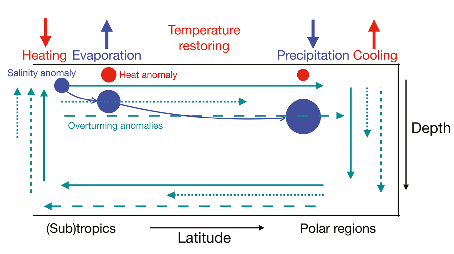
Figure 1: Sketch to describe the mechanism of the Loop Oscillation. A positive salinity anomaly is propagating with the MOC. While it is in the evaporating region, it weakens the MOC, remains longer in this region and hence is amplified. Next, in the precipitating region, it strengthens the MOC, is shorter in this region and is amplified. Moreover, because of different damping of temperature and salinity anomalies, temperature-induced density anomalies appear, which are out of phase with those caused by salinity and hence cause the oscillatory nature of the variability. The timescale is determined by the propagation time of the salinity anomaly over the loop defined by the MOC (details in Sevellec et al. 2006). |
Can this variability be traced back to the amplification of a single pattern in a more idealized model? Indeed, while investigating instabilities of the MOC in an idealized North Atlantic basin, it was found that buoyancy anomalies, which propagate over the overturning loop can be amplified (Sevellec et al. 2006); such oscillations are called "Loop Oscillations" (or overturning oscillations). The mechanism as deduced from such idealized models is sketched in Figure 1 and described in the caption. Similar patterns were also determined in global ocean models, where the timescale of variability is multi-millennial (Weijer and Dijkstra 2003).
Southern Ocean Centennial Variability
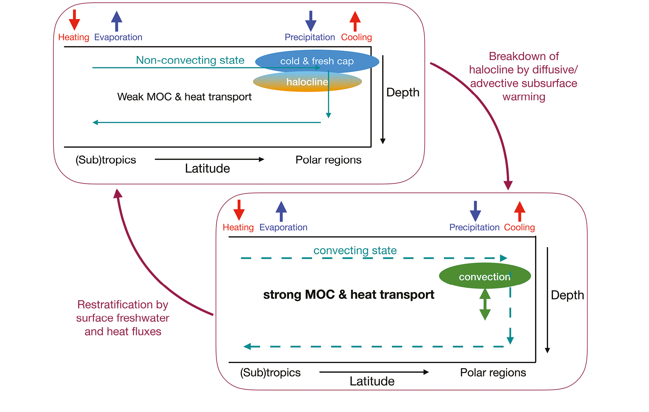
As a second example, we consider the centennial variability which was found in a 1500-year-long simulation with the Kiel Climate Model (KCM) using present-day constant forcing conditions (Latif et al. 2013). The observable used is the Southern Ocean Centennial Variability (SOCV) index, defined as the zonally and meridionally (from 50-70°S) averaged SST anomaly. The SOCV shows centennial variability above the red noise background. For this type of variability convection in the Weddell Sea is crucial with responses on sea-ice extent and MOC in turn affecting the convection.
 |
|
Figure 2: Sketch to describe the mechanism of the Convection-Restratification variability. Starting in a non-(or weakly) convecting state, advective (wind-driven) or diffusive warming of the subsurface ocean causes convection and breaks down the halocline. The convective state increases the strength of the MOC. Through advective and/or diffusive heat and salt fluxes, restratification occurs, which in turn reduces the density at the surface waters eventually causing the transition back to the non-convective state (details in Winton 1995). |
Can this variability again be attributed to a single pattern in a simplified model? In this case, this is more difficult and no single pattern in an idealized model has been found causing this type of variability. However, there are idealized models showing the variability caused by transitions between convective and non-convective states. These changes can therefore best be described by "Convection-Restratification" variability; when the restratification takes place through diffusive processes, the variability has been called a deep-decoupling oscillation or a "flush" (Winton 1995). A sketch of the mechanism of the "Convection-Restratification" variability is given in Figure 2 (with a description in the caption). Here the timescale is dependent on the processes restoring the stratification. When this process is vertical, mixing the timescale is millennial (Colin de Verdiere 2007), but when faster processes of restratification are involved, the timescale can decrease to centennial, or even (multi)-decadal (e.g. LeBars et al. 2016).
A way forward
The two mechanisms described above form the basic mechanisms of centennial variability in either the Atlantic or the Southern Ocean. In other model simulations, variants or modifications are found as the atmosphere and sea-ice components are also affected. At the moment, it is difficult to falsify these basic mechanisms by the observational database. It is therefore important that specific falsification criteria for the mechanisms are developed, which can then be applied every time the database of observations is updated. Also, more sophisticated (nonlinear) data-analysis techniques may be needed to look at higher-order statistics than just simple linear stationary statistical measures (Mukhin et al. 2015). An increasing observational database and good falsification criteria of specific mechanisms are the way forward to get more clarity on the processes responsible for centennial climate variability.
affiliation
Institute for Marine and Atmospheric research Utrecht, Department of Physics, Utrecht University, The Netherlands
contact
Henk A. Dijkstra: h.a.dijkstrauu.nl
references
Charney JG, DeVore JG (1979) J Atmosph Sci 36: 1205-1215
Colin de Verdiere A (2007) J Phys Oceanogr 37: 1142-1155
Cook ER et al. (2000) Clim Dyn 16: 79-91
Delworth TL, Zeng F (2012) Geophys Res Lett 39: L13702
Deser C et al. (2010) Annu Rev Mar Sci 2: 115-143
Hasselmann K (1976) Tellus 28: 473-485
Latif et al. (2013) J Clim 26: 7767-7782
LeBars et al. (2016) Geophys Res Lett 43: 2101-2110
Mukhin D et al. (2015) Sci Rep 5: 15510
Sevellec F et al. (2006) J Mar Res 64: 355-392
Sicre MA et al. (2008) Quat Sci Rev 27: 2041-2047
Shevchenko I, Berloff P (2015) Ocean Mod 94: 1-14
Van der Vaart PCF et al. (2000) J Atmos Sci 57: 967-988
Robert E. Kopp1, A. Dutton2 and A.E. Carlson3
An increasing number of studies reveal regional or global sea-level instability during interglacial periods, belying a traditional assumption of stability. Sea level may have undergone multi-meter-scale variability during the Last Interglacial period, and decimeter-scale variability in the late Holocene.
The scientific community has traditionally considered sea level to be more variable during glacial periods, subject to abrupt millennial-scale changes in climate and glacial dynamics than during warm interglacial periods, thought to be characterized by comparatively stable sea levels. That paradigm is now shifting. Recent reconstructions suggest that sub-millennial, multi-meter-scale oscillations in sea level occurred during the Last Interglacial period and that decimeter-scale variability occurred during the mid to late Holocene in both relative- and global mean sea level.
Last Interglacial sea-level variability
 |
|
Figure 1: Sea-level reconstructions proposed for the Last Interglacial period (not to precise scale). Different interpretations have been made regarding the number of sea-level peaks, though several suggest evidence for one or multiple sea-level oscillations on millennial timescales. |
The stability of Last Interglacial sea level is still debated, with various reconstructions suggesting between one and four distinct global sea-level peaks (Dutton et al. 2015; Fig. 1). Various reconstructions of local or global mean sea level have interpreted as global mean sea-level oscillations in the order of one to several meters in magnitude, occurring over 1-2 ka (Blanchon et al. 2009; Kopp et al. 2013; Rohling et al. 2008; Thompson et al. 2011). Multiple sea-level peaks have been interpreted from the planktic δ18O records of the Red Sea (Rohling et al. 2008). However, the uncertain age constraints on marine sediment records make it challenging to assess rates on 1-2 ka timescales, and the age model for this reconstruction has been modified several times (e.g. Grant et al. 2012). Though the potential local sea-level oscillations seen in the Red Sea record are intriguing, similar oscillations seen in the Holocene portion of the Red Sea record are not considered to represent actual changes in global mean sea level, leaving the interpretation of this variability open to debate.
Other reconstructions with radiometric chronologies are primarily derived from fossil coral reefs that grew near the sea surface. Given the limited precision of dating techniques for the Last Interglacial period, the identification of centennial-scale variability may well remain elusive, but it should be possible to resolve millennial-scale changes. The challenge here lies more in the vertical uncertainty related to paleo-water depth of the corals, raising questions as to whether the apparent sea-level variability in some records may be due to variable paleo-water depths or changes in coral ecology rather than local sea level itself. This demands future work to incorporate a more rigorous assessment of coral assemblages and sedimentary features to interpret sea-level variations, along with the fundamental observations of changes in elevation and time recorded by fossil coral archives. However, other sedimentary features, such as erosional or exposure surfaces in these reef sequences, seem to support multi-meter-scale variability during the Last Interglacial period (Hearty et al. 2007). Despite the interpretation of multiple peaks in sea level at several fossil coral reef sites around the globe, the lack of a consensus in the number, magnitude and timing of such oscillations between individual studies and sites complicates a definitive interpretation of a global sea-level history. Nonetheless, numerous fossil reef sites clearly record at least two stratigraphically distinct generations of reef growth. These generations of reef growth often also display significant differences in their post-depositional diagenesis and coral taphonomy that would support the interpretation of a different post-depositional history before the reefs were exposed during the last glacial cycle (Blanchon et al. 2009; Dechnik et al. 2017).
While it is premature to provide a definitive answer regarding the number of sea-level peaks during the Last Interglacial or the rates of sea-level change associated with these millennial-scale sea-level oscillations, the body of evidence points towards a more variable sea-level history than in the Holocene. Of all contributors to sea-level change, only changes in ice sheets seem to have the potential to explain the inferred multi-meter-scale changes. Existing ice-sheet evidence points towards a monotonic retreat of the Greenland ice sheet that can explain only a fraction of the overall sea-level highstand (Colville et al. 2011); data on the Antarctic ice sheet is inconclusive.
Middle to Late Holocene sea-level variability
In general, Holocene sea-level reconstructions have considerably less uncertainty both in time and the magnitude of changes, and hence are more likely to be able to resolve finer details in sea-level changes. Holocene sea-level proxy records are more abundant than in past interglacial stages, and considerable effort has gone into developing standardized databases that enable formal statistical analysis at both regional (e.g. Engelhart et al. 2015) and global (e.g. Kopp et al. 2016) scales.
Following the end of the final wastage of last ice-age ice sheets at ~7 ka, Holocene sea-level rise slowed overall but continued to rise into the late Holocene, reflecting continued retreat of the Antarctic ice sheet (Ullman et al. 2016). In the late Holocene, the highest-precision proxies are derived from salt-marsh sediments and microfossil assemblages, which can yield decimeter-scale vertical resolution and century- or sub-century-scale temporal resolution. Taking advantage of the compilation of well-structured regional and global databases, Bayesian statistical methods have been used to both develop continuous records at individual locations and also estimate the overall spatio-temporal field of relative sea level at regional (e.g. Engelhart et al. 2015) and global scales (e.g. Kopp et al. 2016). Over the last two thousand years, a statistically identified common global sea-level signal exhibits decimeter-scale fluctuations that partially correlate with reconstructed global-mean surface temperature. Notably, a ~0.2°C global-mean surface cooling over 1.0-0.6 ka (Marcott et al. 2013) coincides with a 0.2±0.2 mm a-1 global sea-level fall leading into the "Little Ice Age". The division of this sea-level fall between ocean thermal contraction and cryospheric growth is uncertain.
Into the Anthropocene
 |
|
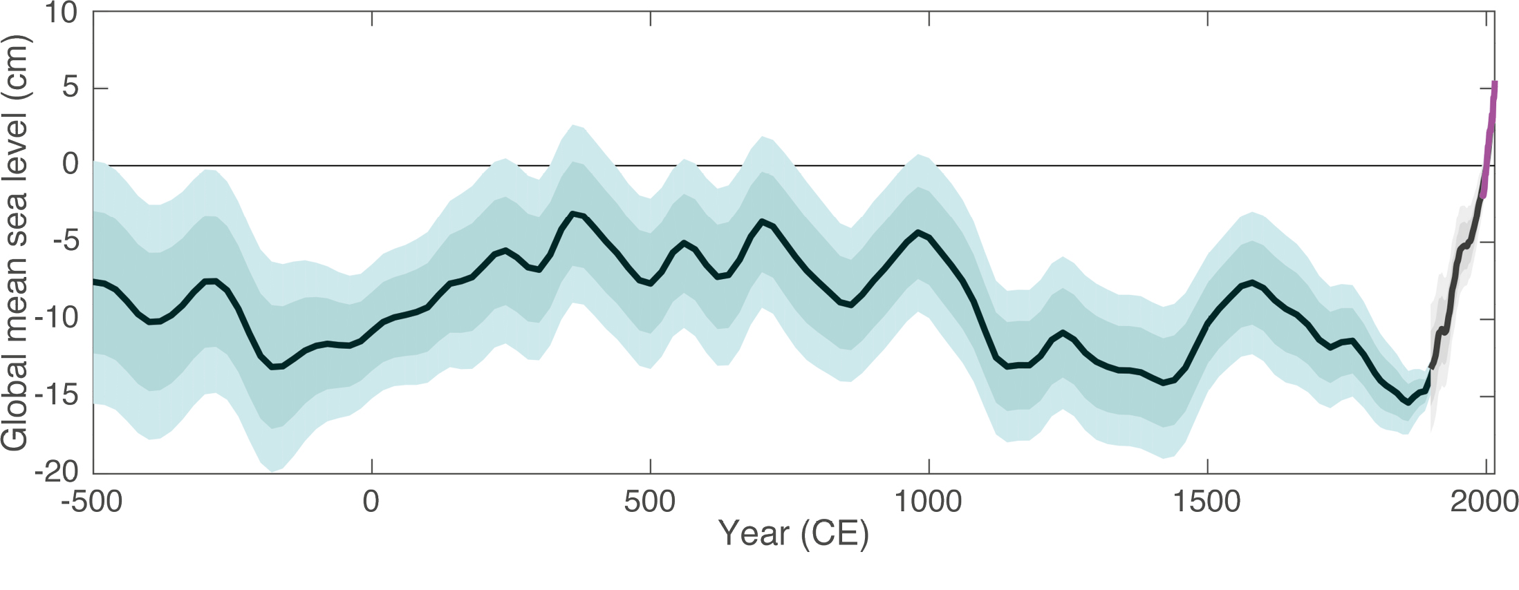
Figure 2: Global-mean sea level over the last 2.5 ka, based on the statistical synthesis of proxy data from Kopp et al. (2016; blue), the tide-gauge-based reconstruction of Hay et al. (2015; grey), and the satellite altimetry record (magenta). Heavy/light shaded regions are 67% and 95% credible intervals. |
A significant global sea-level acceleration began in the late-19th century, with a global sea-level rise of 0.4±0.5 mm a-1 over 1860-1900 CE (Kopp et al. 2016). At a regional scale, the timing of the sea-level acceleration varies broadly, with emergence above the rate of change due to glacial-isostatic adjustment occurring in the 19th century in some areas and the 20th century in others. In the 20th century, global sea level rose at a rate of about 1.4±0.2 mm a-1 (Hay et al. 2015; Kopp et al. 2016) – faster than during any century since at least 2.7 ka (Fig. 2).
The end of the Little Ice Age and the near-synchronous expansion of coal combustion in the 19th century make it challenging to disentangle natural and anthropogenic factors in late-19th and early-20th century sea-level rise. Using the relationship between global mean temperature and global-mean sea level over the last two millennia, Kopp et al. (2016) estimated that, without warming, 20th century global-mean sea level would extremely likely have been limited to -0.4 to +0.8 mm a-1 – leaving between 40 and 130% of the observed rise attributable the effects of twentieth-century global warming. The global-mean sea-level signal of warming emerged at the 95% probability level by 1970 CE.
The ~3 mm a-1 of global-mean sea-level rise since the early 1990s (Hay et al. 2015) has brought the world outside the realm of late-Holocene experience. With global-mean surface temperature now close to that of the Last Interglacial period (Hoffman et al. 2017), researchers have speculated that the world may be committed to long-term global mean sea-level rise comparable to the Last Interglacial period’s 6-9 m peak elevation. Might we also see a return to the enigmatic multi-meter, millennial sea-level dynamism that may have characterized that stage?
affiliations
1Institute of Earth, Ocean and Atmospheric Sciences, Rutgers University, New Brunswick, USA
2Department of Geological Sciences, University of Florida, Gainesville, USA
3College of Earth, Ocean, and Atmospheric Sciences, Oregon State University, Corvallis, USA
contact
Robert E. Kopp: robert.kopprutgers.edu
references
Blanchon P et al. (2009) Nature 458: 881-884
Colville E et al. (2011) Science 333: 620-623
Dechnik B et al. (2017) Global Planet Change 149: 53-71
Dutton A et al. (2015) Science 349: aaa4019
Engelhart SE et al. (2015) Quat Sci Rev 113: 78-92
Grant KM et al. (2012) Nature 491: 744-747
Hay CC et al. (2015) Nature 517: 481-484
Hearty PF et al. (2007) Quat Sci Rev 26: 2090-2112
Hoffman JS et al. (2017) Science 355: 276-279
Kopp RD et al. (2013) Geophys J Int 193: 711-716
Kopp RE et al. (2016) PNAS 113: E1434-E1441
Marcott SA et al. (2013) Science 339: 1198-1201
Rohling EJ et al. (2008) Nat Geosci 1: 38-42
Mathieu Casado, A. J. Orsi and A. Landais
Ice core water stable isotopes are a favored proxy to reconstruct past climatic variations. Yet, their interpretation requires calibration from other proxy records and is affected by various processes which alter the signal after it has been imprinted.
The isotopic composition (δ18O, δ17O and δD) of snow is linked to the condensation temperature because of fractionation associated with distillation from the evaporation site to the precipitation site (Dansgaard 1953). Over large ice sheets, ice is preserved for thousands of years (EPICA 2004) and, thus, analyzing the isotopic composition of the successive layers provides continuous, high-resolution indicators of past climatic variations.
A classical way to retrieve temperature from isotopic composition is to use the spatial relationship between δ18O of surface snow and surface temperature (e.g. Lorius and Merlivat 1975, for Antarctica). However, one should keep in mind two main limitations when using such a method. First, it assumes that the spatial relationship between δ18O and temperature is a good surrogate for the temporal relationship between δ18O and temperature although this link is known to change with time. Second, post-deposition processes affect the snow stratigraphy and the isotopic composition of the snow after precipitation. In the end, the produced time series are also modulated by variable depth-to-time transfer function due to accumulation variations, ice thinning and diffusion.
Resolution and noise
The local accumulation is a determining factor for both the extent of an ice-core record and the maximal resolution that can be achieved. As the ice thickness is capped between 3 and 4 km, depending mainly on the geothermal flux and the topography, it is necessary to choose a site with low accumulation to obtain an ice record spanning several glacial-interglacial cycles (Fischer et al. 2013).
For sites with low accumulation, the snow is exposed at the surface for a long time. Hence, the initial precipitation signal is modified by local post-deposition processes (Ekaykin et al. 2002) due to snow-air interactions, such as the impact of metamorphism, wind and surface roughness, and diffusion. It prevents proper recording of the signal at the intra-seasonal and seasonal scale for sites with accumulation lower than 8 cm ice equivalent per year (Münch et al. 2016).
Deeper in the firn, diffusion smooths the isotopic composition time series, erasing part of the climatic signal (Johnsen 1977). This limits the interpretation of ice-core records at timescales smaller than a few decades.
 |
|
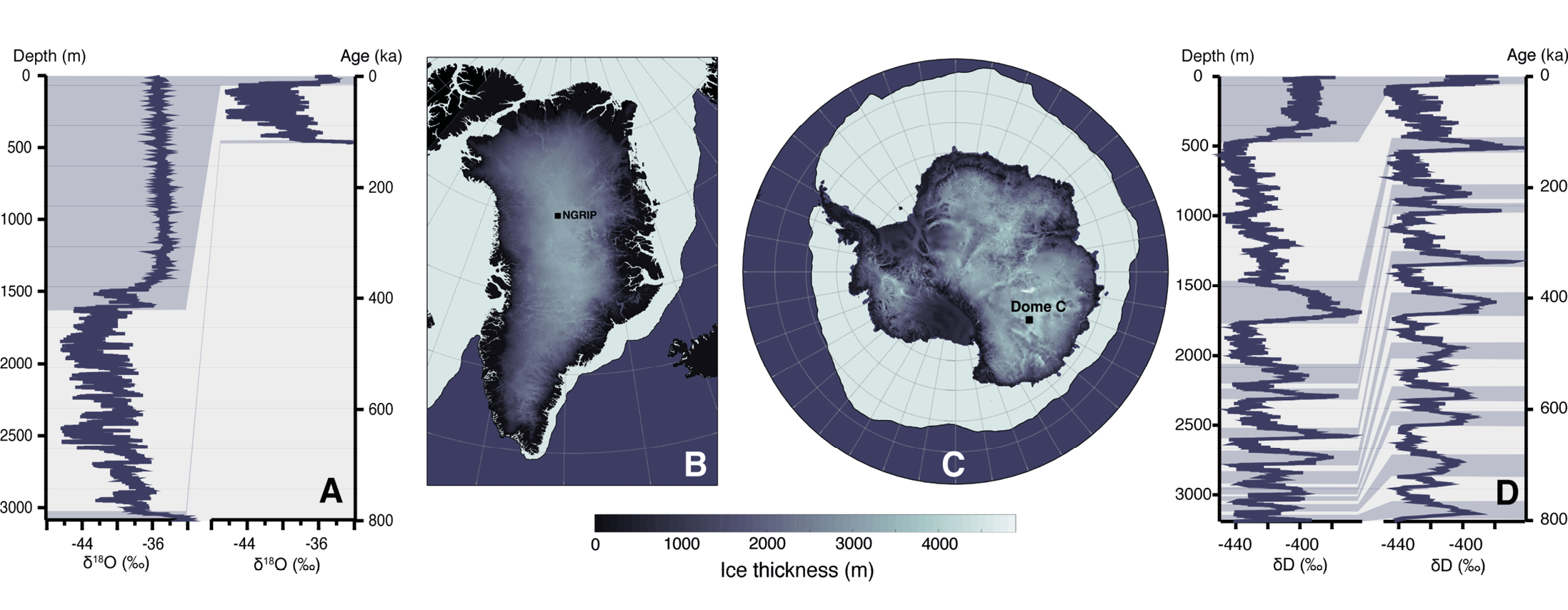
Figure 1: Greenland and Antarctic ice-core sites. (A) Isotopic signal from the NGRIP ice core. (B) and (C) maps of ice thickness in Greenland and Antarctica, respectively. (D) isotopic signal from the Dome C ice core. |
Finally, for longer timescales (and thus deeper in the ice), the varying depth-to-age transfer function affects the spectral properties of the isotopic composition. The first limitation is the accumulation rate itself, which decreases during glacial periods as a thermodynamic response to temperature decrease. The temporal resolution also gets lower with depth due to ice thinning. As illustrated in Figure 1, the number of years per meter globally increases with the depth of the record, from roughly 20 years per meter at the top of the core at Dome C, up to 1400 years per meter for glacial periods at the bottom. Overall, the variability found in single ice-core records combines both the climate variability and several signatures of the archiving process itself.
Isotope to temperature calibration
The calibration of δ18O to temperature can be tested against independent temperature time series, such as borehole measurements at the ice-core site. These measurements performed in Greenland have suggested that the use of the spatial slope (measurements made through space) to estimate the amplitude of the temperature change between the last glacial maximum (LGM) and present-day underestimates by a factor of two the true amplitude of the temperature change (Cuffey et al. 1994). Jouzel et al. (2003) also showed using simulations that the temporal slope (measurements made through time) linking isotopic composition to temperature is less steep than the spatial one and that it does not remain constant over time. This large variability can be due to differences in the large-scale atmospheric circulation, vertical structure of the atmosphere, the seasonality of precipitation, modification of location, or climatic conditions in the moisture source regions.
To take into account the changes in processes involved in the formation of the isotopic signal, calibration of the isotopic paleothermometer is realized through different methods. Weather station data are used at the seasonal and interannual scale, borehole temperature measurements are used at the scale of the recent anthropogenic warming (Orsi et al. 2017) or for the LGM-Holocene transition, and isotopes of nitrogen and argon can be used during abrupt warming events in Greenland (Guillevic et al. 2013). Isotope-enabled climate models can also be used to infer the isotope-temperature relationship with a direct control on the timescale and on the period: for instance, Sime et al. (2009) highlighted that for warm interglacial conditions, the isotope-temperature relationship can become non linear whereas it is not the case for cooler (glacial) conditions.
 |
|
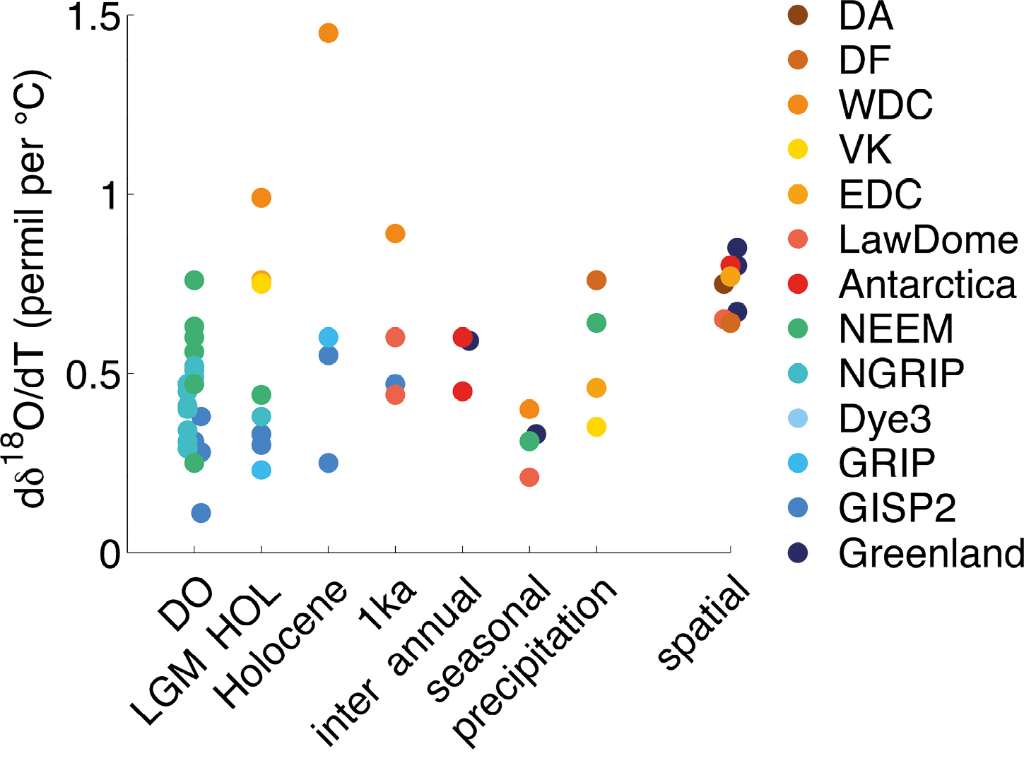
Figure 2: Slopes between isotopes and temperature for different locations and timescales. |
The ensemble of slopes δ18O versus temperature found in the literature (Fig. 2) shows, at all timescales, a large span of values ranging from 0.2 to 1.5‰ °C-1 which differs from the mostly constant spatial slopes. From this compilation, it is clear that neither the seasonal temporal slope nor the spatial slope, which are the most direct to measure, can be used to calibrate the relationship for longer time periods. For instance, work on Dansgaard–Oeschger events (abrupt warming events during glacial periods typically spanning from decadal to centennial scales) showed that, even for events of a similar timescale, at the same site, the scaling is not preserved (Guillevic et al. 2013). This shows that a more complex framework than simple linear regression to temperature is necessary to interpret the isotopic signal.
These variations in the temperature sensitivity need to be properly taken into account before stacking cores from different sites, or computing power spectra, as the respective amplitude of different spectral peaks of δ18O variability may include more than one driver (climatic or not).
Conclusions
If water isotopes from ice-core records are insightful tools to reconstruct past climates, there are fundamental limits to their power of reconstruction.
First, the resolution of the ice-core record is not constant in time, due to changes in the accumulation rate, thinning due to ice flow, post-deposition processes, and diffusion of the water isotope signal in snow and ice. Spectral properties of ice-core water isotopes time series are thus affected. For instance, for low accumulation sites, such as those found on the East Antarctic Plateau (below eight cm per year, ice equivalent), multi-decadal resolution at best can be extracted for the isotopic signal, even for recent periods, whereas in Greenland, where larger accumulation is found, seasonal cycles can be retrieved for the last 1000 years from ice-core records.
Second, the relationship between isotopes and temperature is not constant in time and space. As a result, different methods should be applied to calibrate the isotopic paleothermometer: e.g. borehole temperature for glacial-interglacial transition (millennial scale) or δ15N for rapid climatic variations (decadal to centennial scales).
These observations call for a more careful use of isotopic records when these timeseries are used for general inferences about the climate system (e.g. Huybers and Curry 2006), keeping in mind the variety of processes involved in the archiving of the climatic signal in the snow isotopic composition. Several approaches can help to clearly identify the transfer function leading to the isotopic signal from ice-core records: isotope-enabled global climate models are the way forward to refine the relationship between precipitation δ18O and temperature (Sime et al. 2009), and field studies (Casado et al. 2016) can help evaluate how this signal is modified after the deposition and how the isotope-to-temperature relationship is altered at the seasonal and interannual timescales. Finally, using proxy system models can help quantify the impact of archival processes on the climate signal (Evans et al. 2013).
affiliations
Laboratoire des Sciences du Climat et de l’Environnement, Université Paris-Saclay, Gif-sur-Yvette, France
contact
Mathieu Casado: mathieu.casadogmail.com
references
Casado M et al. (2016) Atmos Chem Phys 16: 8521-8538
Cuffey KM et al. (1994) J. Glaciol 40: 341-349
Dansgaard W (1953) Tellus 5: 461-469
Ekaykin AA et al. (2002) Ann Glaciol 35: 181-186
EPICA (2004) Nature 429: 623-628
Evans MN et al. (2013) Quat Sci Rev 76: 16-28
Fischer H et al. (2013) Clim Past 9: 2489-2505
Guillevic M et al. (2013) Clim Past 9: 1029-1051
Huybers P, Curry W (2006) Nature 441: 329-332
Johnsen S (1977) Proc Symp on Isotopes and impurities in snow and ice, Grenoble 1975, 118: 210-219
Jouzel J et al. (2003) J Geophys Res Atmos 108(D12): 4361
Münch T et al. (2016) Clim Past 12: 1565-1581
Anne de Vernal
Sea-ice observations cover only a few decades, making proxy reconstructions a necessity to document natural variability. Proxy data suggest resilient sea ice in the Canadian Arctic, but large variations in seasonal extent in the Pacific Arctic and subarctic Atlantic.
Sea ice is an important component of the climate system as it is responsible for Arctic amplification through ice-albedo feedbacks and because it controls the exchanges of heat and gas at the ocean-water interface. Sea-ice formation and melt vary in response to incoming energy and depend upon stratification and thermal inertia in the upper water layer, which are functions of salinity. They also vary in space in relation with surface-ocean and atmospheric currents that form pack ice in convergence zones and redistribute sea ice in subpolar seas.
 |
|
Figure 1: Map of the Arctic Ocean with limit of minimum sea-ice-cover extent (mean from 1980 to 2000; minima of 2012 and 2007), main currents paths (white arrows) and location of cores used to illustrate the circum-Arctic sea-ice-cover variations during the Holocene (Fig. 2). |
Satellite observations of Arctic sea ice are continuous since 1979. They show large variations of Arctic sea-ice extent at intra-annual timescales, from summer (September ~6.3±1.1 106 km2; see limit in Figure 1) to winter (March ~15.5±0.5 106 km2), which represent about 60% of the change in the coverage (see http://nsidc.org/data/seaice_index). Beyond seasonal variation, a multidecadal decreasing trend is recorded, with a larger change in summer (13.3% per decade) than winter (2.7% per decade). The decrease in summer sea-ice extent is correlated with the rise of surface air temperature (r2~0.63). However, the sea-ice decline is non linear and could result, at least in part, from internal variability (Swart et al. 2017). Longer-than-satellite time series are therefore needed for a proper assessment of trends and to document the full range of sea-ice variability under natural forcings and feedbacks.
Reconstructing past sea ice
The development of time series covering centuries to millennia is a challenge. Among approaches used to document past sea ice, one consists of the compilation of historical archives such as ship logs, diaries and any sea-ice-related observations (e.g. ACSYS 2003). Available information encompasses a few centuries and mostly covers the subarctic North Atlantic where human populations have settled. It illustrates variations in seasonal extent of sea ice in areas located along the winter-spring sea-ice edge, with multidecadal variations, for example in the Barents Sea (Vinje 2001), or the secular trend since the 19th century, for example off Iceland (Lamb 1977). The data also show clear regionalism, which point to complex dynamics of the seasonal sea ice and prevent spatial extrapolation from isolated sites.
Another approach to reconstruct Arctic sea-ice extent uses its relationship with climate to derive time series based on the analysis of annually resolved climate-related data from tree rings and ice cores of circum-Arctic regions (Kinnard et al. 2011). This approach allowed for the development of a comprehensive 1400-year record of late summer Arctic sea-ice extent, which suggests natural variability ranging mostly from ~9 to 11 106 km2 (Kinnard et al. 2011). The set of data is, however, heterogeneously distributed with very rare data points from the Russian Arctic, which is the most critical region with respect to the recent decline in sea-ice cover.
 |
|
Figure 2: Reconstructed sea-ice cover versus ages during the Holocene. The thin lines correspond to estimates and the thick lines are the smoothed values, which better illustrate millennial-scale variations. |
Most studies to document past Arctic sea ice on a long timescale use biogenic proxies from marine sediment cores, based on the assumption that sea ice controls environmental conditions such as light, temperature and salinity, thus playing a determinant role on species’ distribution, primary productivity and biogenic fluxes to the sea floor (de Vernal et al. 2013a). Microfossils routinely recovered in marine sediments, such as ostracods or foraminifers, were used as paleoceanographic tracers, but their relationship to sea ice is indirect (e.g. Cronin et al. 2010; Polyak et al. 2013). Among marine microorganisms yielding microfossil remains, diatoms and dinoflagellates appear to be more directly related to sea ice as they include taxa associated with sea ice. For example, some diatom species blooming in spring sea ice produce organic biomarkers (IP25), providing direct indications on sea-ice occurrence (e.g. Belt et al. 2007). Many IP25 time series have been produced since 2007, but the curves remain qualitative in the absence of calibration (e.g. Belt and Müller 2013; Stein et al. 2017). Quantitative estimates of sea-ice cover were proposed from transfer functions based on the calibration and the application of modern analogue techniques. In particular, regional data sets of diatom distributions in the surface sediments were used to quantitatively estimate spring sea-ice concentrations from transfer functions, notably in the eastern Baffin Bay (Sha et al. 2014). Hemispheric-scale databases of dinoflagellate cyst populations allowed the application of modern analogue techniques for quantitative reconstructions of seasonal sea ice at many sites in the Arctic and subarctic seas (de Vernal et al. 2013b; See examples in Fig. 2).
The limitation of marine sea-ice proxies
Regardless of the approach, the marine-based sea-ice records suffer from several caveats:
(1) The temporal windows of proxy-data. A sediment slice (1 cm usually) may represent decades to centuries or millennia, depending on sedimentation rates (mm per year to cm per thousand years) and bioturbation. This is problematic in the central Arctic Ocean where accumulation rates are particularly low.
(2) The "modern" relationships between the proxies and sea ice are defined from the comparison of surface sediment samples and recent observations, which usually do not encompass the same time window. This is an important source of errors when calibrating transfer functions and applying modern analogue techniques.
(3) Each record has first a local to regional value. The spatial distribution of marine-core records of past sea ice is not dense enough for extrapolation at the scale of the Arctic Ocean and subarctic seas. The rarity of quantitative sea-ice estimates in the Russian Arctic, where the largest variability is presently recorded, is a critical issue.
(4) Year-round ice-free conditions and seasonal sea ice can be assessed from many proxies, but perennial or multiyear sea ice is more difficult to reconstruct. One ostracod taxon parasite of sea-ice nematode was used to assess multiyear sea ice in the central Arctic (Cronin et al. 2013), but perennial ice cover is usually deduced from negative evidence (nil productivity of primary producers).
Circum-Arctic sea ice during the Holocene
Despite limitations, the marine data provide clues on sea-ice cover variations with time windows ranging from decades to centuries, thus yielding smoothed records. At the scale of the Holocene, proxy-data suggest limited variations in general, with likely resilient perennial sea ice in the central Arctic Ocean, but greater variations in the seasonal sea ice as expressed in terms of spring sea-ice concentration (Sha et al. 2014) or number of months of sea ice (de Vernal et al. 2013b) in the Arctic and subarctic seas which are within the limits of winter sea ice. In other words, the variability of sea-ice cover as reconstructed from marine proxies illustrates more the seasonality of its extent and concentration than the actual changes in the Arctic-wide extent of sea ice. The amplitude of local changes during the mid- and late Holocene seems to be mostly comprised within the range of interannual variations as recorded during the last decades. At some sites, variations from a dominant mode to another (low to high sea ice) is recorded with a pacing ranging from multidecadal to millennial scales that may, however, depend upon the time resolution achieved by the analyses. The records based on a standardized quantitative approach, allowing comparison at the circum-Arctic scale, show limited changes and persistent sea ice in the Canadian Arctic, but large-amplitude changes closer to the Pacific and Atlantic gateways (de Vernal et al. 2013b; Fig. 2), where inter-basin exchanges (freshwater and heat fluxes) seem to result in a higher variability in sea ice cover. They also suggest diachronous, if not opposite, changes in the western (Pacific) Arctic versus eastern (Atlantic) Arctic at millennial scales, which might well illustrate shifts from dominant Arctic dipole pattern (Wang et al. 2009) to strong polar vortex leading to more stable Arctic sea-ice cover.
affiliation
GEOTOP, Université du Québec à Montréal, Canada
contact
Anne de Vernal: devernal.anneuqam.ca
references
Belt ST et al. (2007) Org Geochem 38: 16-27
Belt ST, Müller J (2013) Quat Sci Rev 79: 9-25
Cronin TM et al. (2010) Quat Sci Rev 29: 3415-3429
Cronin TM et al. (2013) Quat Sci Rev 79: 157-167
de Vernal A et al. (2013a) Quat Sci Rev 79: 1-8
de Vernal A et al. (2013b) Quat Sci Rev 79: 111-121
Kinnard C et al. (2011) Nature 479: 509-512
Lamb HH (1977) Climate History and the Future, vol. 2. Methuen, 835 pp
Polyak L et al. (2013) Quat Sci Rev 79: 145-156
Sha L et al. (2014) Palaeogeogr Palaeoclimatol Palaeoecol 403: 66-79
Stein R et al. (2017) J Quat Sci 32: 362-379
Swart NC et al. (2017) Nat Clim Change 5: 86-89