PAGES Magazine articles
Dominique Genty1, S. Verheyden2 and K. Wainer3
We present a review of 13 speleothems from Europe, Asia and South America, covering the penultimate deglaciation and the last interglacial. We highlight the similarities and regional differences in the growth rate and the calcite δ18O records in these cave deposits.
The discovery of speleothems (cave calcite deposits) as paleoenvironmental archives has significantly enriched the toolbox for reconstructing past changes over the continents. Indeed, research over the last decade has demonstrated the potential of speleothems for providing unique paleoenvironmental and paleoclimatic information based on: (1) precise chronologies relying on Uranium-series dating and (2) high-resolution continental climate records based on carbon and oxygen isotope (δ13C and δ18O respectively) measurements of the calcite.
Among other results, speleothems have revealed that the Asian and South American monsoons show an anti-phase pattern (Cruz et al. 2005; Cruz et al. 2006a) paced by Earth's precession changes (Wang et al. 2001; Wang et al. 2008). In the Northern Hemisphere temperate zone, the millennial scale climatic Dansgaard-Oeschger events occurring frequently over Marine Isotopic Stage 3 (28-60 ka BP) have been detected in stalagmites from Turkey (Fleitmann et al. 2009), from the Austrian Alps (Spötl and Mangini 2002), and from southwestern France (Genty et al. 2003). This non-exhaustive list of results gives a flavor of how speleothem records complement other terrestrial evidence, e.g. from lake sediments (Allen et al. 1999; Brauer et al. 2000) or pollen (Sanchez Goñi et al. 2002; Sanchez Goñi et al. 2008).
 |
|
Figure 1: Geographical locations of the selected speleothems. |
In particular, speleothems enable significant advances in providing precise age determination over the penultimate deglaciation (Termination II) and the last interglacial (LIG) period. Could speleothems provide a continuous, well-dated, and well-understood reference record for Termination II? We review the speleothem δ18O records covering Termination II and the LIG that satisfy the following criteria: (1) They should be characterized by a high density of Uranium-Thorium (U-Th) ages of high precision (i.e. 2σ age error < 1-5%), (2) the speleothems should have a high enough growth rate so that samples for U-series dating cover a time interval shorter than the uncertainty of the age, and (3) growth rates should be continuous over long periods avoiding long hiatuses. Following these criteria, we selected seven records from Asia (Fig. 1): four from the Sanbao Cave (China; Wang et al. 2008), two from the Dongge Cave (China; Kelly et al. 2006; Yuan et al. 2004) and one from the Daeya Cave (Korea; Jo et al. 2011). From South America, we selected two records from Brazil. They were retrieved in the Botuvera Cave (Cruz et al. 2005; Cruz et al. 2006b) and in the Santana Cave (Cruz et al. 2006a). We further considered six records from European/Mediterranean caves (Fig. 1) located in Corchia (Italy; Drysdale et al. 2005; Drysdale et al. 2009), La Chaise (France; Couchoud et al. 2009), Entrische Kirche (Austria; Meyer et al. 2008; Meyer et al. 2012), Villars (France; Wainer et al. 2011), Maxange (France; Genty and Wainer unpublished) and Soreq (Israel; Bar-Matthews and Ayalon 2002). While various parameters have been measured on speleothems such as calcite δ13C and trace elements, we focus here only on the δ18O signal of the calcite and its growth-rate.
Calcite δ18O
 |
|
Figure 2: A) Calcite δ18O and growth rate records for European speleothems and calcite δ18O record for a Middle East speleothem. B) Calcite δ18O and growth rate records for Asian and South-American speleothems. |
Several environmental factors influence the sensitivity of the calcite δ18O to rainfall δ18O and/or temperature (McDermott 2004). Firstly, changes in the location of the water vapor source, in the source’s isotopic composition, and also changes in rainfall amount influence the calcite δ18O. This results in lower δ18O when the climate is more humid and warmer, e.g. as shown by monsoon speleothem records and the Corchia record in Italy (Cruz et al. 2006a; Drysdale et al. 2005; Jo et al. 2011; Wang et al. 2008; Fig. 2). Secondly, the temperature in the cave (close to the mean annual external temperature) may also have a significant influence on the calcite precipitation fractionation, and consequently on the calcite δ18O (i.e. δ18O decreases when temperature increases), as suggested in the Villars stalagmite (e.g. Genty and Wainer unpublished; Wainer et al. 2011). Thirdly, changes in the seasonality of precipitation (e.g. the proportion of winter versus summer precipitation) can influence the calcite δ18O in specific cases such as in the Entrische Kirche Cave record (Meyer et al. 2008, 2012) where the seasonality effect drives the increase of calcite δ18O over Termination II while the climate continues to warm (Fig. 2A).
Speleothem growth rate
The speleothem growth rate is also a key parameter for climatic reconstruction. The calcium content of the dripping water and the drip rate mainly control the growth rate. Those two factors are influenced by climatic conditions (e.g. external temperature, precipitation) and soil and vegetation activity (Baker et al. 1998; Dreybrodt 1988). As a consequence, the records from densely U-Th dated speleothems generally reveal a close link between growth rate and calcite δ18O (Fig. 2). Within a single stalagmite, the growth rate can vary from a few µm yr-1 during cold and dry periods to more than 1 mm yr-1 during warmer and more humid climate phases. The chronology can, therefore, only be constrained if a high number of precise dates can be generated on an as small as possible time interval.
We observe that all the low-latitude stalagmites from Asia and South America grew continuously over Termination II (Fig. 2B), while in Europe only the Corchia stalagmite seems to present such a progressive growth (i.e. with no hiatus) (Fig. 2A). Unfortunately, the low growth-rate in the Corchia speleothem, less than 30 mm of calcite deposition from its base at ~170 until ~129 ka BP, limits the acquisition of multiple precise ages over Termination II. Chronological limitations also exist for Entrische Kirche, Maxange, and La Chaise stalagmites, which started to grow during or just after Termination II and a hiatus is visible in the Villars record before 130 ka BP (Fig. 2A).
Termination II and LIG records
Figure 2 shows the calcite δ18O and growth-rate records from the selected speleothems. We observe that (1) most of the European speleothems started growing between 132 and 122 ka BP and all display an abrupt increase in growth rate during a short period: between ~129.7 and ~125.8 ka BP (Fig. 2A). On the contrary, the onset of Asian and South-American speleothem deposition and/or growth rate increase is more scattered and ranges from ~138 to ~123.4 ka BP (Fig. 2B). (2) Interestingly, while δ18O records show roughly similar changes concentrated around 130 ka in Europe and in Asia, the growth rate changes are much more important in European samples than in low latitude ones (Asia, South America). This suggests that the climatic contrasts between cold and warm phases of the deglaciation are different between mid-latitude and low-latitude regions. (3) The Corchia record, through its comparison with the MD95-0242 marine sediment core (Drysdale et al. 2009), suggests the start of termination II at 141 ka ±2.5 ka. This is only slightly marked by the calcite δ18O and the growth rate curves. No comparable transition signal at this age is found in Asian speleothems, which on the contrary, display a δ18O increase interpreted as a weakening of the Asian monsoon. However, a major transition is clearly visible in the Corchia record in both the calcite δ18O and growth rate, between ~131.5 ka and ~128.5 ka. Additional well-dated speleothems are urgently needed to shed light on the timing of the onset of Termination II in Europe compared with Asia. (4) A good agreement between the Corchia and La Chaise records is observed for the timing of the LIG climatic optimum and the calcite δ18O (~128 ka BP ± 1). However, the calcite δ18O from Villars Cave, which is geographically closer to La Chaise Cave than the Corchia Cave, reveals a different shape over the LIG and lower calcite δ18O values. Interestingly, the Villars calcite δ18O amplitude change over Termination II has a similar magnitude to the record from the Soreq cave located in the Middle East.
This comparison clearly reflects (1) different regional responses to climate forcing and (2) region- and site- specific controlling factors of the calcite δ18O values.
Concluding remarks
Speleothem time-series have become an invaluable terrestrial archive to reconstruct climate changes. The δ18O records and the growth rate curves discussed here show an abrupt and general warming onset between ~129.7 and 125.8 ka BP in Europe. Under a monsoon climate regime, we observe also an abrupt variation in the δ18O records. However the growth rate curves are much more scattered (i.e. between ~138 and ~123.4 ka BP) suggesting a less marked climatic transition. New data gathered in the framework of the Past4Future project (see Verheyden et al. this issue) should enable us to clarify the observed regional differences over the LIG. In addition, the increasing speleothem demand will certainly need a coordinated and internationally referenced sample management system in order to minimize the impact on cave preservation.
acknowledgements
We warmly thank the authors who made their data available to construct the figures.
affiliations
1Laboratoire des Sciences du Climat et de l’Environnement, CEA Saclay, Gif-sur-Yvette, France dominique.genty lsce.ipsl.fr
2Geological Survey, Royal Belgian Institute of Natural Sciences, Belgium
3Department of Earth Sciences, University of Oxford, UK.
Selected references
Full reference list online under: pastglobalchanges.org/products/newsletters/ref2013_1.pdf
Cruz FW et al. (2006a) Earth and Planetary Science Letters 248: 495-507
Drysdale RN et al. (2009) Science 325: 1527-1531
Wainer K et al. (2011) Quaternary Science Reviews 30: 130-146
Emilie Capron1, A. Landais2, P.C. Tzedakis3, E. Bard4, T. Blunier5, D. Dahl-Jensen5, T. Dokken6, R. Gersonde7, F. Parrenin8, M. Schulz9, B. Vinther2 and C. Waelbroeck2
We review some of the available strategies for a coherent dating of ice, marine, and terrestrial records from various latitudes over the last interglacial.
Within the Past4Future project, specific efforts are dedicated to the improvement of absolute age scales and to the synchronization of climate records from different archives and different latitudes. A specific committee has been set up to develop guidelines for dating and synchronization to help with synthesizing and integrating results from the Work Packages that produce and compare the datasets.
While the Holocene is relatively well dated, the last interglacial (LIG) lasting approximately from 129 to 118 ka BP, has been attributed different durations depending on the considered records (e.g. Kukla et al. 1997; Shackleton et al. 2002). These differences result from regional disparities and dating inconsistencies (Dutton and Lambeck 2012). Building a reference timeframe for the LIG is thus essential to disentangle climatic external forcing and internal feedbacks as well as to depict the regional sequences of events.
Here, we review some of the existing absolute constraints and synchronization strategies over the LIG for providing a coherent stratigraphic framework to present paleoclimatic records. We also provide an example of developing a common timescale for marine and ice core records over the LIG using approaches discussed below. The list of age markers discussed hereafter is not exhaustive but the complete document established by the Past4Future dating committee is available at http://www.past4future.eu/index.php/resources/project-resources (M5.1.2 Workshop: Integration of results, 2012).
Absolute age markers
 |
|
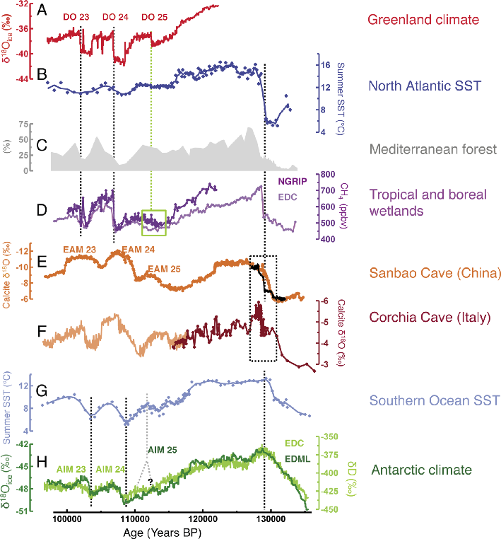
Figure 1: A) NorthGRIP δ18Oice (NorthGRIP Project members, 2004), B) Summer Sea Surface Temperature (SST) from ODP 980 marine core (Oppo et al. 2006), C) Temperate tree pollen percentages from MD95-2042 marine core (Shackleton et al. 2002), D) Atmospheric methane concentrations from NorthGRIP (Dark purple, Capron et al. 2010) and EDC (Light purple, Loulergue et al. 2008) ice cores, E) Speleothem δ18O from Sanbao Cave (orange, Wang et al. 2008; black, Cheng et al. 2009), F) Speleothem δ18O from Corchia Cave (brown, Drysdale et al. 2007; light orange, Drysdale et al. 2009), G)Summer SST from MD02-2488 marine core (Govin et al. 2012), H) EDC δD (Jouzel et al. 2007) and EDML δ18Oice (EPICA community members, 2006). All records are synchronized onto the EDC3 timescale except the speleothem records. Dashed lines highlight the unambiguous tie points used to synchronize marine records onto ice core records (Govin et al. 2012). The green rectangle and dashed line highlight the ambiguous signature of GIS 25 onset in the NorthGRIP methane concentration record (Capron et al. 2012). The black dashed rectangle highlights that the abrupt δ18Ocalcite shift over Termination II is not synchronous in the various speleothem records. The yellow areas indicate the divergence between ice core and speleothem records in the age of Dansgaard-Oeschger (DO) events 23, 24, and 25. The grey dashed lines point to the AIM 25 event as identified in the EDC (Jouzel et al. 2007) and in the EDML (Stenni et al. 2010) water isotopic profiles and illustrates the difficulty to define unambiguous pointers over the glacial inception. |
Speleothems provide absolute ages of climate events thanks to dating methods based on Uranium-series. For example, the largest increase of the Asian Monsoon activity (as reflected in the Sanbao speleothem abrupt calcite δ18O decrease) over the penultimate deglaciation (Termination II) occurred at 129 ka BP with an associated error of less than 100 years (Cheng et al. 2009; Fig. 1E). For European speleothems, less abundant in Uranium, dating constraints are usually less precise (e.g. Genty et al. 2003).
The upper parts of ice cores in high-accumulation areas can be dated by identifying and counting annual layers (e.g. Svensson et al. 2008). However, ice cores lack deep and old absolute dating horizons except for tephra layers. To date, only the absolute dating of the tephra from Mount Moulton volcanic event provides an absolute age constraint at 92.1 ±4.4 ka BP (Dunbar et al. 2008) included in the EPICA Dome C timescale (hereafter, EDC3 timescale; Parrenin et al. 2007). In order to place additional constraints, orbital tracers (δO2/N2, air content, δ18Oatm) have been implemented for ice core timescales (e.g. Dreyfus et al. 2007; Kawamura et al. 2007; Parrenin et al. 2007; Raynaud et al. 2007). But because the mechanisms behind these orbital tracers are yet to be fully understood (e.g. Landais et al. 2012; Dreyfus et al. 2007), the associated uncertainties are large (e.g. 6 ka for δ18Oatm).
A close inspection of the last glacial inception and the succession of Greenland Stadials (GS) and Interstadials (GIS) reveals significant differences in the timescales of the onset of GIS 23, 24 and 25 as recorded in NorthGRIP δ18Oice (Fig. 1A) and their counterparts in speleothem records from Corchia Cave (Drysdale et al. 2007, Fig. 1F) and Sanbao Cave (Cheng et al. 2009; Wang et al. 2008; Fig. 1E).
Record synchronization
Ice core synchronization is done on (1) the ice phase through identification of the same volcanic events (e.g. Parrenin et al. 2012) or 10Be variability from different ice cores (Raisbeck et al. 2007), and (2) the gas phase through global atmospheric tracers (methane concentration, δ18Oatm, e.g. Blunier et al. 1998, Fig. 1D).
For example, a chronology for the EPICA Dronning Maud Land (EDML) ice records, coherent with the EDC3 timescale (as illustrated with the EDML and EDC water isotopic profiles on Figure 1H) has been developed by synchronizing volcanic horizons and dust peaks from the EDML ice with EDC ones (Ruth et al. 2007; Severi et al. 2007). Subsequently, the NorthGRIP record has been put on the EDC3 age scale synchronizing the abrupt changes in CH4 concentration (Fig. 1D) and δ18Oatm variations linked to the DO events between 70 and 123 ka BP (Capron et al. 2010). However, this synchronization exercise has some limitations when clear methane concentration or δ18Oatm signatures are lacking (e.g. Capron et al. 2012; Fig. 1D, green square).
Direct correlation of the plateau of benthic foraminifera δ18O minimum values is commonly applied for synchronizing marine sediment records during the LIG (e.g. Cortijo et al. 1999). However, this method has limitations when considering records from different water depths and oceanic basins (Skinner and Shackleton 2005; Waelbroeck et al. 2011). An alternative synchronization approach would be based on the identification of tephra layers in marine sediment with a similar chemical composition (e.g. Rasmussen et al. 2003).
Changes in the Earth’s magnetic field intensity are recorded in marine, terrestrial, and ice records (e.g. Raisbeck et al. 1987). While absolute dating of tephra layers and speleothems allow attribution of an absolute timescale to the Earth’s magnetic field variations, the latter can then be used to link the various archives (e.g. Zhou and Shackleton 1999).
Climatostratigraphic alignment
While it is desirable to use global markers or joint analyses of different proxies within the same physical sequence (e.g. dust measured both in ice and marine cores), relative dating can sometimes only be derived indirectly from climatic records. Climatostratigraphic alignment is inevitably based on assumptions about the mechanisms linking climate and measurements. These underlying hypotheses have to be explicitly formulated.
Possible alignments between marine and ice core records are based on the hypothesis that Sea Surface Temperature (SST) changes in the sub-Antarctic zone of the Southern Ocean (respectively in the North Atlantic) occurred simultaneously with air temperature changes over inland Antarctica (respectively Greenland) (e.g. Govin et al. 2012; Shackleton et al. 2002). Figure 1 (A-B, D, G-H) illustrates how this approach can produce a coherent relative timescale between marine and ice core records from both hemispheres (Govin et al. 2012). Age pointers were defined at the start of Termination II and over the millennial-scale events identified towards the end of the LIG (Fig. 1A-B, G-H). However, regional disparities in climatic event expression lead to a relative uncertainty of up to 1 ka (Buiron et al. 2012). Also, it remains problematic to define precise tie points within the LIG (Govin et al. 2012) and one should limit the use of tie points to unambiguous climatic features.
At a regional scale, marine SST and speleothem records may be aligned on the principle that variations in regional SSTs, air temperatures, evaporation and moisture transport are synchronous, and ultimately affect speleothem δ18O signatures (e.g. Drysdale et al. 2009). These changes in moisture availability and air temperature should also affect synchronously terrestrial ecosystems. Such an approach could potentially be used to align speleothem and pollen records at the start and end of the LIG and within the LIG.
Cheng et al. (2006) suggested that abrupt calcite δ18O shifts from Chinese speleothems correlate to sharp methane concentration changes measured in ice cores that are associated with abrupt climate changes from the last glacial period and the last two climatic terminations. This hypothesis has been used to constrain the EDC3 timescale over Termination II (Parrenin et al. 2007; Fig. 1D, E, H). However, the interpretation of speleothem δ18O and δ13C in terms of climatic or environmental parameters is not straightforward (e.g. Baker et al. 1997). In particular, the climatic interpretation of Chinese stalagmite δ18O has been recently challenged (Pausata et al. 2011; Wang and Chen 2012). Also, the question as to whether rapid calcite δ18O variations measured in Chinese speleothems are systematically synchronous with abrupt methane concentration increases requires further investigation (Fleitman et al. unpublished data).
Perspectives
The guidelines for dating and synchronization established so far aim for moving toward a coherent LIG dating. Within that context, a coherent timescale between several ice and marine records from both hemispheres has already been established (e.g. Capron et al. 2010; Govin et al. 2012).
Matching various paleo-records also requires assessing rigorously the coherence of the different dating methods and developing integrated techniques. For example, the EDC3 timescale will be replaced soon by AICC2012, a new Antarctic Ice Core Chronology derived from an inverse model that integrates and optimizes absolute and new relative constraints from several ice cores (Bazin et al. 2012).
The guidelines will be updated as new higher-resolution records emerge that may allow for increasing the number of chronological tie points over past interglacials through the identification of additional rapid events and the use of improved radiometric techniques (e.g. Aciego et al. 2010).
affiliations
1British Antarctic Survey, Cambridge, UK; ecapbas.ac.uk
2Laboratoire des Sciences du Climat et de l’Environnement, CEA Saclay, Gif-sur-Yvette, France
3UCL Department of Geography, University College London, London, UK
4Centre de Recherche et d’Enseignement de Géosciences de l’Environnement, Aix en Provence, France
5Department of Geophysics, University of Copenhagen, Denmark
6Bjerknes Center Centre for Climate Research, Bergen, Norway
7Alfred Wegener Institute, Bremerhaven, Germany
8Laboratoire de Glaciologie et Géophysique de l’Environnement, Grenoble, France
9MARUM, Center for Marine Environmental Sciences, and Faculty of Geosciences, University of Bremen, Germany
Selected references
Full reference list online under: pastglobalchanges.org/products/newsletters/ref2013_1.pdf
Capron E et al. (2010) Quaternary Science Reviews 29: 222-234
Cheng H et al. (2009) Science 236: 248-252
Govin A et al. (2012) Climate of the Past 8: 483-507
Parrenin F et al. (2007) Climate of the Past 3: 485-497
Shackleton NJ, Hall MA, Vincent E (2000) Paleoceanography 15: 565-569
Louise C. Sime1, V. Masson-Delmotte2, C. Risi3 and J. Sjolte4
We present new atmospheric isotope simulations in order to investigate the effect of sea surface temperature changes on the relationship between Greenland surface temperature and water isotopes.
Recently, ice core scientists have obtained for the first time a Greenland ice core record covering the entire last interglacial (LIG; Dahl-Jensen this issue; NEEM community members 2013). Previously, ice cores drilled in Greenland have shown that the stable water isotopic value (δ18O) of LIG ice at fixed elevation was enriched relative to present day, with a maximum enrichment across central Greenland regions of at least +3‰ at 126 ka BP (e.g. NorthGRIP Project members 2004). This +3‰ enrichment has been interpreted as indicating LIG Greenland warmth, but also lower LIG ice sheet topography or warmth outside of Greenland. Thus, achieving a better understanding of the regional drivers of Greenland precipitation δ18O is of broad interest to the ice core and wider paleoclimate communities.
LIG forcing versus greenhouse gas driven warming
In the framework of the Past4Future project, two recent papers have used atmospheric isotope enabled General Circulation Models (GCM) to investigate climatic controls on δ18O measured in Greenland ice cores. Each paper has focused on a specific modeling approach.
The first approach uses simulations from the IPSL-CM4 model to simulate the LIG climate using realistic boundary conditions, i.e. 126 ka BP orbital configuration and greenhouse gas (GHG) levels (Masson-Delmotte et al. 2011). The second approach (also preliminarily investigated in Masson-Delmotte et al. 2011) is as follows: First, two different warm sea surface temperature (SST) scenarios are simulated using the IPSL-CM4 and HadCM3 GCMs forced with high GHG values (see Box 1). Second, the impact of the two SST scenarios on isotopic changes over Greenland is simulated with the respective isotope-enabled atmosphere-only versions of IPSL-CM4 and HadCM3 (Sime et al. 2013). Hereafter, we refer to these three simulations as: (1) IPSL_LIG: IPSL-CM4 LIG simulation driven by 126 ka BP orbital and 126 ka BP GHG forcing; (2) IPSL_A: IPSL-CM4 simulation using present day orbital forcing alongside higher levels of GHG forcing and (3) HadCM3_B: HadCM3 simulation using present day orbital forcing alongside higher levels of GHG forcing (Box 1).
 |
|
Figure 1: Scaled differences between the control (present day) and the warmer simulations. Climate and isotopic results are scaled such that central Greenland δ18O increases by +3‰. (A) IPSL_LIG simulation, (B) IPSL_A simulation and (C) HadCM3_B simulation. Shading over Greenland shows the difference between the control and individual simulation values of surface temperature. Contouring shows the difference between the control and individual simulation values of δ18O. Intervals are 2‰ and the range is from 0 to 12‰. Figure from Sime et al. (submitted) |
To facilitate simulation inter-comparison, we firstly average the simulated δ18O increases over central Greenland (regions above 1300 m). We then linearly scale the results so that the three simulations each have a 3‰ increase in δ18O compared with present day (Fig. 1). This enables a direct comparison between simulated temperature increases over Greenland, and SST changes that could force the observed LIG 3‰ δ18O increase. Although observationally based (NorthGRIP Project members 2004), the target of an average of +3‰ in LIG δ18O is somewhat arbitrary. It may not be necessary for the δ18O increase to average 3‰ across all central regions of Greenland in order to match all interglacial ice core observations. The SST changes simulated within IPSL_A and HadCM3_B also have a degree of arbitrariness, i.e. alternative patterns of SST changes could also drive up Greenland δ18O values.
 |
|
Figure 2: Differences between the control (present day) and warmer simulation SSTs. Scaled (as in Fig. 1). (A) IPSL_LIG simulation, (B) IPSL_A simulation and (C) HadCM3_B simulation. The viewpoint in each case is from above Europe, looking across the North Atlantic Ocean, Greenland, and part of the Arctic Ocean. Schematic arrows show the main changes in precipitation (evaporation) sources for Greenland snow. |
A broad comparison between simulations shows that IPSL_LIG and IPSL_A SST patterns differ where orbitally-dependent seasonal behavior occurs (Fig. 2A-B). However, these differences appear to be smaller than those observed between the purely GHG (orbits as present day) forced IPSL_A and HadCM3_B experiments (Fig. 2B-C).
What surface temperature changes drive a +3‰ increase in δ18O?
For Greenland, above 1300 m, the scaled IPSL_LIG simulation suggests an averaged interglacial surface temperature increase greater than 14°C. However it also features "cliff-edges" in δ18O and surface temperature (Fig. 1A). IPSL_A simulates an interglacial Greenland surface temperature increase of ~10 to 14°C (Fig. 1B) while HadCM3_B simulates an interglacial Greenland surface temperature increase of ~2 to 8°C (Fig. 1C). For the IPSL_A and HadCM3_B simulations, the surface temperature and δ18O changes tend to be larger in the northern and central regions of Greenland compared to present day (Fig. 1B and 1C).
The "cliff-edge" pattern across Greenland from the IPSL_LIG simulation indicates "simulation noise", and scaling to the +3‰ target requires SST increases that are not within observational bounds (Fig. 2A; McKay et al. 2011; Turney et al. 2010). Thus, despite the appeal of the 126 ka BP simulation (IPSL_LIG) approach, we suggest that climate model dynamics currently prevent an accurate simulation of LIG climate when using realistic orbital and GHG forcing. These model deficiencies could be due to missing physical processes in the ocean, atmosphere, and sea ice sub-models as well as missing climate feedbacks due to a neglect of dynamic vegetation and ice sheet evolution in the model. This motivates the use of isotopic simulations driven by higher levels of GHGs (such as the IPSL_A and HadCM3_B simulations) when attempting to learn about past warm climates.
We show that understanding SST changes is key to understanding warm climate Greenland isotopic changes (Masson-Delmotte et al. 2011; Sime et al. 2013). Indeed, precipitation sourced from local high-latitude regions is enriched in δ18O. Increasing (decreasing) the proportion of locally sourced precipitation therefore raises (lowers) δ18O in Greenland snow. Thus SST changes which drive differences in evaporative sources, strongly affect Greenland δ18O values. From the results of the IPSL_A simulation, we observe strong SST increases south of 50°N but only small changes around northern Greenland (Fig. 2B). This leads to a higher proportion of distally sourced (δ18O depleted) Greenland precipitation. The HadCM3_B simulation shows that the northern regions of Greenland experience SST increases of up to ~10°C (Fig. 2C), associated with reduced sea ice cover (not shown). This leads to substantially more local precipitation and as a result, enriched ice δ18O.
What can we learn from these results?
Our simulations provide an insight into how ice core observations could be related to wider climatic changes across the North Atlantic and Arctic Oceans. On one hand, we observe from the HadCM3_B simulation that if the seas to the north of Greenland get warmer and sea ice is reduced, then central Greenland δ18O increases of 3‰ (Fig. 1C) can be simulated with associated SSTs of around +4°C (Fig. 2C). This pattern of sea surface warming lies within current interglacial observational constraints (McKay et al. 2011; Turney et al. 2010). On the other hand, the IPSL_A simulation shows that if the Arctic SSTs north of Greenland are almost unchanged and SST warming is instead concentrated in the south of Greenland (Fig. 2B) the 3‰ δ18O rise requires Greenland surface temperatures to increase by between ~8 and 14°C (Fig. 1B). It also requires an SST change to the southeast of Greenland of more than ~20°C (Fig. 2B). Such a large change is very unlikely and this suggests that the warming resulting from the HadCM3_B may be more representative of LIG changes.
To summarize, while during colder than present day climates, Greenland δ18O originates from distal precipitation sources (Masson-Delmotte et al. 2005), our new simulations suggest that during warmer climates, Greenland δ18O precipitation can originate from local high latitude regions. As a result, we propose that sea surface warming and sea ice loss in regions north of Greenland may have caused much of the observed Greenland δ18O rise and also contributed to a central Greenland temperature increase of about +4°C during the LIG. SST reconstructions from marine sediment cores drilled in regions to the north of Greenland would be necessary to test our hypothesis.
Outlook
Our experiments have shown that improved model parameterizations and/or coupling with dynamic ice sheet and vegetation models are necessary for investigating Greenland LIG changes forced by more realistic orbital and GHG forcings. Isotope-enabled model simulations, which include dynamic ice sheets, would also be useful for helping us infer LIG ice sheet changes from isotopic observations. Finally, performing atmospheric isotopic model simulations is also beneficial in understanding other ice core tracers used to interpret Greenland moisture source changes (such as the deuterium excess and the recently developed δ17O tracer).
Box 1: Orbital forcing configuration and greenhouse gas (GHG) values for the three simulations: IPSL_LIG (Masson-Delmotte et al. 2011) IPSL_A, HadCM3_B (Sime et al. 2013)
| Simulation | Orbital forcing | GHGs |
|---|---|---|
| IPSL_LIG | 126 ka | 126 ka |
| IPSL_A | present-day | 4x preindustrial CO2 |
| HadCM3_B | present-day | SRES A1B 2100 scenario |
affiliations
1British Antarctic Survey, Cambridge, UK; lsimbas.ac.uk
2Laboratoire des Sciences du Climat et de l'Environnement, Gif-sur-Yvette, France
3Laboratoire de Météorologie Dynamique, Paris, France
4Lund University, Sweden
references
Full reference list online under: pastglobalchanges.org/products/newsletters/ref2013_1.pdf
Masson-Delmotte V et al. (2011) Climate of the Past 7, 1041-1059
Masson-Delmotte V et al. (2005) Science 309: 118–121
Rainer Gersonde1 and Anne de Vernal2
Past sea ice extension is a critical component of the Earth’s climate system. Reconstructions relying on geochemical, sedimentological and microfossil-based proxy records in ice and sediment climate archives are presented here.
On August 27, 2012 the US National Snow & Ice Data Center (NSIDC, http://nsidc.org/arcticseaicenews/) and the National Aeronautics and Space Administration (NASA, https://www.nasa.gov/topics/earth/features/arctic-seaice-2012.html) alerted the public about the lowest Arctic summertime sea ice extent measured since the satellite-based sea ice survey was started in the late 1970s. The observed August 2012 minimum sea ice extent of 4.1×10⁶ km2 confirms the ongoing decline of perennial Arctic sea ice, which potentially began in the middle of the last century (Kinnard et al. 2008). The decline reached 2 to 3% per decade between 1979 and 1996 and accelerated to 12 to 13% per decade since then (Comiso 2012). This rapid loss of sea ice, higher than anticipated by the forecasts of the IPCC 2007 report (Stroeve et al. 2007), may lead to the disappearance of summer Arctic sea ice by 2050 if not earlier, according to several model simulations (Wang and Overland 2009). Arctic sea ice decline, which is related to Arctic surface water temperature increase (Comiso 2012), represents a striking example of current climate change related to anthropogenic global warming (Spielhagen et al. 2011; Kinnard et al. 2011).
 |
|
Figure 1: (A) Schematic representation of major sea ice related environmental and climatic parameters (adapted from Gersonde and Zielinski 2000). (B) Photo gallery showing the development of Antarctic sea ice (a fast changing environmental factor) from frazil ice (1) to aggregation of ice crystals (2) to form pancake ice (3), freezing and rafting of pancake ice (4, see fur seal for comparison) to form a close ice cover (5, crossed by the German research vessel ice breaker Polarstern). The different steps of this process take only a few days to weeks. Photos: R. Gersonde. |
Although sea ice is generally restricted to high latitudes, its formation, extent and seasonal variability play a critical role in the Earth´s climate and ocean dynamics at global and regional scales, affecting surface albedo, the exchange of energy fluxes between ocean and atmosphere, thermohaline ocean circulation and formation of deep water masses, primary and export productivity, and weather system formation (e.g. Budikova 2009) (Fig. 1A). Sea ice is a fast changing environmental component of the Earth system (Fig. 1B) and effectively amplifies climate and environmental change due to positive feedback mechanisms. The recent changes in Arctic sea ice extent are of concern to scientists and policy-makers, and this topic is regularly reported in the media. Thus we need to further extend sea ice records into the past to document the natural variability of sea ice beyond short term satellite measurements to better understand the recently observed changes and enhance our ability to perform projections of future sea ice extent.
Historical sea ice records
At the hemispheric scale, sea ice reconstructions for historical periods predating the start of satellite surveys are hampered by the lack of observational datasets. Nevertheless, Kinnard et al. (2008) extended the observation-based record of Arctic sea ice back to 1870 AD. This was mainly based on statistical analysis of ice edge position data. The record was then extended to 560 AD based on a high-resolution multi-proxy approach using ice, terrestrial, and marine records. This historical record demonstrates that the observed modern decline of sea ice has been unprecedented for the past 1,450 years (Kinnard et al. 2011). Rayner et al. (2003) simulated Arctic and Antarctic sea ice and their seasonal variability back to 1856 AD, taking into account historical observations and modern climatologies. Their analysis indicates reductions in Antarctic sea ice extent by the middle of the last century; a result supported by a comprehensive study of whaling positions (de la Mare 2009) and ice core proxy records (Abram et al. 2010). Such a finding is puzzling, since satellite-derived information indicates a slight increase in Antarctic sea ice (about 1% per decade) during the past 40 years (Turner et al. 2009).
Sea ice on geological time scales
Sea ice reconstructions on geological timescales rely on indirect observations obtained from marine and ice core records. Various proxies have been developed to estimate sea ice extent, concentration, annual occurrence, and seasonal pattern. However, each proxy has its own limitations. While winter sea ice extent can be reconstructed somewhat accurately with a number of proxies, estimating the extent of the perennial sea ice field remains challenging. Moreover, while the analyses of cores may yield time series at given locations, the reconstruction of sea ice extent in space with the position of maximum and minimum limits requires densely distributed data. Consequently, comprehensive glacial/interglacial reconstructions require combining different proxy records and consideration of sedimentation patterns to map sea ice extent and its variability.
Sea ice proxies include chemical tracers in ice cores and biogenic remains of microorganisms as well as non-biogenic particles in marine records. Flux rates of methanesulfonic acid (MSA) and sea salt sodium in ice cores are used to reconstruct past sea ice extent (e.g. Becagli et al. 2009; Wolff et al. 2006) but their interpretation is equivocal and more studies are needed to understand and calibrate these proxies (Abram et al. 2010). Marine reconstruction methods include the use of microfossil marker species, transfer functions based on microfossil assemblages, stable isotope signals, biomarker and terrigenic particles. Specific diatom species are able to dwell in sea ice, attached to it or within sea ice governed cold-water environments (less than -1.5°C). Some of these species produce biomarkers or secrete siliceous valves that can be preserved in the sediment record. For example, a proxy to reconstruct past Arctic sea ice is the IP25 biomarker (a C25 mono-unsaturated highly branched isoprenoid lipid) (Belt et al. 2007). IP25 is produced by a sea ice-related diatom, which secretes thinly walled siliceous valves generally not preserved in the sedimentary record. To better quantify sea ice occurrence, Müller et al. (2011) have proposed using a combination of IP25 and a phytoplankton productivity proxy. The occurrence of IP25 is restricted to the polar North (e.g. Müller et al. 2009). A similar biomarker has recently been proposed for reconstruction of Antarctic sea ice (Massé et al. 2011).
 |
|
Figure 2: (A) Reconstruction of Antarctic winter and summer sea ice extents during the Last Glacial Maximum based on diatom proxies (blue lines). For comparison modern winter and summer sea ice extents are indicated (green lines). The LGM reconstruction in the Pacific sector and the Drake Passage are weak because of the small number of available cores at the time of data compilation. Dots indicate locations with diatom-based reconstruction, crosses indicate locations with radiolarian-based reconstruction (modified from Gersonde et al. 2005). (B) Reconstruction of sea ice cover in the North Atlantic during the Last Glacial Maximum based on organic walled dinoflagellates. The orange and green dashed lines correspond to the probable limits of summer (perennial) and winter sea ice limits, respectively (modified from de Vernal et al. 2005). |
The abundance pattern of sea ice related diatom species preserved in the sediment record represents a powerful tool for Southern Ocean sea ice reconstruction. While early work (Hays et al. 1976) simply used the boundary of diatom-rich and diatom-poor sediments for the mapping of the sea ice extent at the Last Glacial Maximum (LGM), later studies considered the composition of diatom assemblages and reconstructed sea ice quantitatively as expressed by the annual duration (month per year) of sea ice occurrence using a diatom transfer function (Crosta et al. 1998). A combination of different diatom-based methods allowed the first comprehensive circum-Antarctic reconstruction of the LGM winter and summer sea ice distribution as part of the MARGO project to be realized (Gersonde et al. 2005; Fig. 2A).
In Northern Hemisphere high latitudes, the use of diatoms, however, is often restricted by silica dissolution. Some reconstructions from Quaternary sediments are nevertheless available for the North Atlantic (e.g. Justwan and Koç 2008), the Labrador Sea and the polar North Pacific. In contrast, organic-walled dinoflagellate cysts display a broad distribution pattern and are usually well-preserved in sediment. They have successfully been used for past sea ice reconstructions (e.g. de Vernal et al. 2005, 2008) documenting the LGM sea ice distribution in the North Atlantic (Fig. 2B). Other potentially useful proxies include ostracode species that live parasitically on sea ice-related amphipods (Cronin et al. 2010), the isotopic signature of a sea ice-related planktic foraminifer species (Hillaire-Marcel and de Vernal 2008), and the relationship between sea surface temperatures derived from the planktic foraminiferal assemblage record and sea ice occurrence (Sarnthein et al. 2003). Finally, the application of different sedimentological proxies for reconstruction of Arctic sea ice and its transport pathways has been attempted (Stein 2008). An interesting combination of terrigenic components (ice-rafted debris) and the occurrence of an extinct diatom species, which may be related to an extant sea ice-related diatom genus, has been used for the establishment of a two-million-year sea ice record which occurred in the middle Eocene Arctic Ocean (Stickley et al. 2009).
Outlook
In the framework of the Past4Future project, bipolar reconstructions, derived from several of the proxies described above, are generated to enhance our knowledge of sea ice variability during the present and last interglacial stages and the preceding glacial/interglacial transitions. The challenge to produce time series of sea ice extent into past warmer than present climates and to study natural sea ice variability under such conditions is central to the Sea Ice Proxy (SIP) working group supported by PAGES (de Vernal et al. 2012).
affiliations
1Alfred-Wegener-Institute for Polar and Marine Research, Bremerhaven, Germany; Rainer.Gersondeawi.de
2GEOTOP, Université du Québec à Montréal, Montréal, Canada
Selected references
Full reference list online under: pastglobalchanges.org/products/newsletters/ref2012_3pdf
Belt ST et al. (2007) Organic Geochemistry 38: 16-27
Comiso JC (2012) Journal of Climate 25, doi: 10.1175/JCLI-D-11-00113.1
de Vernal A et al. (2005) Quaternary Science Reviews 24: 897-924
Gersonde R, Crosta X, Abelmann A, Armand L (2005) Quaternary Science Reviews 24: 869-896
Emma J. Stone1, P. Bakker2, S. Charbit3, S.P. Ritz4 and V. Varma5
A last interglacial transient climate model inter-comparison indicates regional and inter-model differences in timing and magnitude of peak warmth. This study reveals the importance of different climate feedbacks and the need for accurate paleodata in terms of age, magnitude and seasonality to constrain model temperatures.
Paleorecords and climate modeling studies indicate that Arctic summers were warmer during the last interglacial (LIG, ca. 130 to 115 ka BP) and global sea level was at least 6 m higher than today (Dutton and Lambeck 2012; Kopp et al. 2009), implying a reduction in the size of the Greenland and Antarctic ice sheets (Siddall et al. this issue). Previous snapshot climate model simulations for the LIG have shown summer Arctic warming of up to 5°C compared with the present day (Kaspar et al. 2005; Montoya et al. 2000), with the largest warming in Eurasia and the Greenland region. The LIG period provides an opportunity to test the current suite of climate models of varying degrees of complexity, under forcings that result in a warmer than present climate. To date, however, there has been no standardized inter-comparison of LIG climate model simulations.
Five European modeling groups (forming part of the Past4Future project) have performed experiments in order to characterize the response of the climate system to LIG changes in various climate forcings and biophysical feedback processes. These forcings and feedbacks include greenhouse gas concentrations (GHG), orbital configuration (ORB), vegetation feedbacks (VEG), and changes in ice sheet geometry (ICE). A key aim of this inter-comparison is to perform a number of sensitivity studies (e.g. ORB only, ORB+GHG, ORB+GHG+VEG, ORB+GHG+ICE) to ascertain the relative importance of the forcings and feedbacks in determining the trends and variability of LIG climate.
The Past4Future project has enabled the first long (> 10 ka) transient standardized inter-comparison for the LIG to be realized. These simulations consist of a range of model complexity with various forcings and feedbacks included: one full general circulation model CCSM3 (ORB; Collins et al. 2006; Yeager et al. 2006), one low-resolution general circulation model, FAMOUS (ORB+GHG; Smith 2012; Smith et al. 2008), and three Earth System Models of Intermediate Complexity: 1) CLIMBER-2 (ORB+GHG; Petoukhov et al. 2000), 2) Bern3D (ORB+GHG+ICE; Müller et al. 2006; Ritz et al. 2011), and 3) LOVECLIM (ORB+GHG; Goosse et al. 2010). CLIMBER-2, Bern3D, FAMOUS, and LOVECLIM use GHG and orbital forcings that conform closely to a set of standards described by the Paleo-modeling Inter-comparison Project (PMIP3) while CCSM3 uses the same orbital configuration but with greenhouse gas values fixed according to mean LIG values. Bern3D is the only model that prescribes ice-sheet changes (and an associated freshwater forcing) by including the effect of remnant Northern Hemisphere ice sheets from the penultimate glaciation (all other models use present day ice sheet geometry).
One of the difficulties in understanding the response of the climate to LIG forcings is the lack of consensus in the paleodata on the timing of peak interglacial warmth in different regions of the Earth (e.g. The Nordic Seas and North Atlantic; Govin et al. 2012; Van Nieuwenhove et al. 2011). The interpretation of temperature signals of different resolution and seasonality obtained from paleoclimatic archives is also contentious (Jones and Mann 2004). Our climate modeling approach aims to inform on the spatial and temporal differences in peak warmth observed in the data, as well as on assessing the robustness of our climate model results (Bakker et al. 2013). Through this task it is also possible to gain an understanding of the climate feedbacks (e.g. changes in ocean overturning circulation and sea-ice) that are at play resulting from changed GHG concentrations and astronomical forcing.
How does LIG summer temperature response compare
in four different regions of the Earth?
 |
|
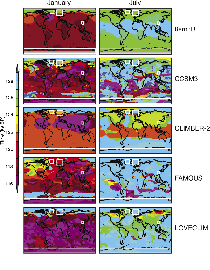
Figure 1: Summer 50-year global mean temperature anomalies spanning the LIG (ca. 130 to 115 ka BP) for five climate models of varying complexity. Note that these anomalies are calculated with respect to a preindustrial equilibrium climate representative of 1850 AD. For more details with respect to model setups and forcings see Bakker et al. (2012). The range in timing of the peak interglacial warmth is indicated by the gray bars. |
Figure 1 shows the 50-year summer average surface air temperature anomalies over four defined regions of the globe where paleodata exist for the time period 130 to 115 ka BP. These model results demonstrate not only the differences in the timing of peak summer warmth between regions but also discrepancies between the models themselves. Greenland shows peak summer warmth during the early LIG for all five models with positive temperature anomalies compared with pre-industrial values ranging from ~0.1 to 1°C, albeit substantially smaller than the +5°C anomaly obtained from ice core records (e.g. NorthGRIP Project members 2004). Future simulations, which include a reduced Greenland ice sheet, may reconcile this difference between models and data.
Simulated maximum summer temperature anomalies for the Nordic Seas (-1.0 to 1.0°C) and southeast China (~0 to 3°C), however, indicate a less robust result between the models in terms of timing and temperature change. We compare our model results with a recent data synthesis by Turney and Jones (2010) and show that no model produces a maximum summer temperature anomaly as large as that inferred from paleodata (up to +9°C) for the Nordic Seas. This discrepancy could be due to missing feedback processes in the model simulations (such as vegetation changes), misrepresentation of ocean circulation and a simplistic representation of sea ice dynamics. Furthermore, the discrepancy could be larger still because the Turney and Jones (2010) data synthesis has been interpreted as an annual rather than a summer temperature signal. We also note that the Bern3D model simulation, which includes remnant ice sheets from the previous glacial, shows a delay in peak LIG warmth for Greenland and the Nordic Seas compared with the other models indicating the importance of this feedback.
In contrast to Greenland, timing of summer peak warmth in the Southern Hemisphere shows a substantial delay, with peak summer values (from -1 to 0.1°C) only being obtained after 120 ka BP. This contradicts a recent paleodata study (Govin et al. 2012) suggesting Southern Hemisphere peak warmth actually preceded Northern Hemisphere warming during the early part of the LIG.
Seasonal timing of LIG maximum warmth
 |
|
Figure 2: Timing of maximum LIG warmth for the months January and July for the five climate models of varying complexity. The regions defined in Figure 1 for Greenland, Nordic Seas, southeast China, and Antarctica are depicted by the white boxes . Figure modified from Bakker et al. (2013). |
Figure 2 shows the spatial distribution of timing of maximum LIG warmth during January and July. Superimposed are the four regions described above and given in Figure 1. During Northern Hemisphere winter (January), there is large variability between models in the timing of maximum warmth ranging from ca. 119 to 128 ka BP over Greenland and the Nordic Seas. We relate these discrepancies at high northern latitudes during winter to differences in sea-ice feedback mechanisms (Bakker et al. 2013). In contrast, Southern Hemisphere winter (July) temperatures over Antarctica show less variability in timing of peak winter warmth. The temperature anomalies reach a maximum ca. 128 ka BP for CLIMBER-2, LOVECLIM and FAMOUS relating to those simulations which include the same forcings. There is a delay in peak warmth for Bern3D and CCSM3 (CCSM3 does not include transient GHGs and Bern3D includes remnant ice sheets and changes in freshwater forcing).
During the northern summer months, the inter-model comparison shows consistent timing of maximum warmth at high latitudes, ranging between ca. 124 and 128 ka BP (Fig. 2). This consistency is also the case for the Southern Hemisphere in July, but austral summer maximum warmth occurs much later (after 118 ka BP). In northern mid-to-low latitude regions, such as southeast China, all model simulations show reasonably similar results in timing of maximum warmth during the northern summer (July) and winter (January) months.
Perspectives
The Past4Future LIG modeling group provides important information for the data community regarding locations for relevant potential new paleoclimatic data. We also provide insights into understanding the mechanisms that result in differences in peak warmth timing and magnitude from proxy data temperatures around the world. Our results inform on the impact of remnant ice sheets and the importance of understanding the sensitivity of climate feedbacks during periods of enhanced warming. Part of the Past4Future data and modeling community remit is to reconstruct a coherent picture of LIG climate with the use of climate models to explain the temperature patterns observed in proxy observations. The next stage will be to take part in a detailed multi-millennial scale temperature comparison between model and data for the LIG. This will aim at understanding and explaining the differences between climate model results and how they might constrain future predictions of global warming.
affiliations
1School of Geographical Sciences, University of Bristol, UK emma.j.stonebristol.ac.uk
2Earth & Climate Cluster, Department of Earth Sciences, Vrije Universiteit Amsterdam, The Netherlands
3Laboratoire des Sciences du Climat et de l'Environnement, CEA Saclay, Gif-sur-Yvette, France
4Climate and Environmental Physics, Physics Institute and Oeschger Centre for Climate Change Research, University of Bern, Switzerland
5Center for Marine Environmental Sciences and Faculty of Geosciences, University of Bremen, Germany
Selected references
Full reference list online under: pastglobalchanges.org/products/newsletters/ref2013_1.pdf
Bakker P et al. (2013) Climate of the Past 9: 605-619
Govin A et al. (2012) Climate of the Past 8: 483-507
NorthGRIP Project members (2004) Nature 431: 147-151
Turney CSM, Jones RT (2010) Journal of Quaternary Science 25: 839-843
Van Nieuwenhove N et al. (2011) Quaternary Science Reviews 30: 934-946
Thomas Blunier1, J. Chappellaz2 and E. Brook3
New techniques have revolutionized the way trace gases are measured from ice cores. What took decades to complete in the past now only takes a few months. We report about the recent development in measuring the methane concentration from ice cores.
 |
|
Figure 1: Methane concentration variations over the last 100 ka. (A)Composite record from several Greenland ice cores (Blunier et al. 2007), (B) Raw data obtained with the SARA (green curve) and Picarro laser spectrometers (red curve). This data is preliminary, uncalibrated, and for illustrative purposes only. It is known to contain sections with analytical issues. |
Ice cores provide a unique opportunity to access the past composition of the Earth’s atmosphere. Up to now methane concentration measurements have been made on individual ice samples. Such work is laborious and it took two decades to obtain the methane data for the composite record shown in Figure 1A.
Initially chemical measurements were also obtained from individual ice samples. During the 1990s a methodology known as Continuous Flow Analyses was invented and has been further developed since (Bigler et al. 2011; Kaufmann et al. 2008). This method is based on the continuous melting of a section of the ice core. The meltwater is then split and diverted into detectors specific to the chemical ion species to be analyzed. In this way a large range of chemical components can be analyzed directly at the ice core drill site. Note that for these chemical measurements, a debubbler unit is required to remove the air from the ice (on the order of 10% by volume) since the air would hamper the chemical analysis. It has been a long-term ambition to measure the gas composition of ice cores using a similar methodology. The University of Bern, Switzerland, has developed such a system.
First in-the-field methane concentration measurements
The system, developed in Bern, is based on a small portable Gas Chromatograph for methane concentrations (Schüpbach et al. 2009). The debubbler unit has been modified so that the expelled air is routed through a membrane unit to separate the air from the remaining water. The membrane unit consists of a hydrophobic membrane tube where the outside of the tube is flushed with ultrapure Helium. The air passes through the membrane and is taken up by the Helium stream. The Helium/air sample mixture is then dried and transferred through a column trap held at the temperature of liquid nitrogen to concentrate the air sample. Finally, this air sample is injected into the Gas Chromatograph. This new way of measuring ice core air composition has proven successful and produces a measurement at ~15 cm intervals along the core with a measurement uncertainty of 3%, i.e. sufficient to reveal the main features of atmospheric methane concentration changes (Schüpbach et al. 2009). Still, the resolution potentially achievable is limited by the requirement to (1) pre-concentrate the sample and (2) separate the trace gases chromatographically.
Introduction of laser spectrometers to ice core works
The research teams at LGGE (Laboratoire de Glaciologie et Géophysique de l'Environnement, Grenoble, France) and CIC (Centre for Ice and Climate, Copenhagen, Denmark) have independently developed the use of cavity enhanced laser spectrometry for obtaining methane concentration measurements. Whilst the LGGE group has made improvements to a prototype instrument (SARA) in collaboration with a laser physics research laboratory at Grenoble (LIPhy, http://www-lsp.ujf-grenoble.fr/SARA-Analyzer-laser-of-traces-of), the CIC group has adapted a commercially available Picarro instrument for the specific requirement of ice core analysis.
During the 2009 NEEM deep drilling campaign, the CIC scientists made the first attempt to couple a Picarro instrument to the existing Bern Continuous Flow Analyses setup. The instrument was connected to the outlet of the Gas Chromatograph gas trapping system in order to measure the sample diluted in Helium. This setup was initially unsuccessful due to the variable dilution of the sample but it demonstrated that laser instruments could be successfully used in the field. Furthermore, initial tests indicated that it would be possible to obtain reliable results if gas concentration measurements were made on the undiluted flow.
Success during the NEEM 2010 field season
 |
|
Figure 2: Schematic of the NEEM 2010 field setup for measuring methane concentrations. |
During the 2010 field season, the project was expanded and included two laser instruments backed up by the Gas Chromatograph system (Fig. 2). LGGE and CIC researchers developed a way of extracting the gas in the melt stream without diluting the sample using a Membrana MicroModule unit and the setup was modified such that the gas/water stream from the debubbler unit was routed directly through the membrane unit. On the gas side of the membrane the air extracted from the ice was pumped through a drier to remove water vapor and then successively through the SARA and Picarro analyzers (Fig. 2). Figure 1 shows the composite of several Greenland ice core methane concentration records obtained over the last 20 years (Fig. 1A) and the raw methane concentration data obtained from the respective laser spectrometers (Fig. 1B). In just two months of using the laser spectrometers the teams were able to obtain measurements that previously took two decades to perform.
Although the system was regularly calibrated with a standard gas, there are obvious differences and inconsistencies between the records. These arise from leaks in the setup and from incomplete gas extraction. For the 2010 records the only way to calibrate the data was to measure some individual samples. While, in principle, the measurements should be continuous, they were in fact broken up into sections of 1.1 m. At the beginning of each section the cavities of the spectrometers are filled with standard gas, which is then slowly replaced with sample gas. Over the course of time in places where sample and standard gas coexist in the cavity the methane concentration of the sample cannot be measured, and in the 2010 setup up to one third of the sample was lost, resulting in only some sections being continuously measured for their methane concentration.
Since 2010, there has been continuous development and improvement in the sample calibration procedure. We now receive good data getting the system into a dynamical steady state situation. In this way solubility correction and eventual leaks are constant and identical for calibration measurements and samples. The precision of the laser systems is significantly better than that of a Gas Chromatograph system with an uncertainty as small as 0.4%.
Stowasser et al. (2012) investigate to what degree the time resolution of methane records can be improved by continuous measurements. Atmospheric variations are smoothed by traveling through the open porous space (firn) in the top part of the ice sheet (the first ~60-100 m) before the gas becomes trapped permanently in the ice. To obtain the full resolution of the smoothed concentration record trapped in the ice, the dispersion by the measurement system has to be less than the smoothing that occurs in the firn layer. The CIC system obtains a spatial resolution of 5 cm, which is adequate to detect any climatically relevant fluctuations in methane back to at least 66 ka BP in the NEEM ice core.
The significant advantage of the online gas concentration measuring technique is the higher resolution that can be obtained in a very short amount of time. This is especially true for the last millennium and part of the Holocene where the system enables a sub-annual temporal resolution on the NEEM ice core to be obtained. At first glance this ability is meaningless, as the atmospheric variations (e.g. annual fluctuations) are completely smoothed out, but we also found indications of sub-annual methane signals in the NEEM ice core. These signals could point to either in-situ production of methane in the NEEM ice or, alternatively, an artifact of the trapping process of air in the firn layer (e.g. stratigraphic inversions due to firn layers trapping gases at different depths) (Rhodes et al. unpublished data). Future investigations are necessary to clarify these issues.
Outlook
Laser spectrometer development has rapidly improved over the past few years. In the future it will be possible to analyze not only one atmospheric component such as the methane concentration described here, but a suite of atmospheric components simultaneously. This has already been achieved by the SARA instrument, which has measured both methane and carbon monoxide on a section of the NEEM ice core. Within the framework of the Past4Future project, online measurements of trace gases will be able to supply climate models with the most complete dataset to date.
affiliations
1Centre for Ice and Climate, Niels Bohr Institute, University of Copenhagen, Denmark; bluniergfy.ku.dk
2Laboratoire de Glaciologie et Géophysique de l’Environnement, CNRS, Université Joseph Fourier-Grenoble, France
3Department of Geosciences, Oregon State University, Corvallis, USA
Selected references
Full reference list online under: pastglobalchanges.org/products/newsletters/ref2013_1.pdf
Bigler M et al. (2011) Environmental Science and Technology 45: 4483-4489
Blunier T et al. (2007) Climate of the Past 3: 325-330
Kaufmann PR et al. (2008) Environmental Science and Technology42: 8044-8050
Schüpbach S et al. (2009) Environmental Science and Technology 43: 5371-5376
Stowasser C et al. (2012) Atmospheric Measurement Techniques 5: 999-1013
Mark Siddall1, R.C.A. Hindmarsh2, W.G. Thompson3, A. Dutton4, R.E. Kopp5 and E.J. Stone6
The Last Interglacial Global Mean Sea Level is believed to be 6 to 9 m above the present and might have two distinct maxima. Here, we discuss the possible fluctuations and their implications for ice sheet evolution.
The duration and timing of the Last Interglacial (LIG) Global Mean Sea Level (GMSL) fluctuations are active areas of research, with distinct features of this sea level change increasingly being reproduced in diverse datasets and syntheses (Dutton & Lambeck 2012; Kopp et al. 2009; Thompson et al. 2011). We review and discuss these possible changes in LIG GMSL and, in particular, what we may infer from them in terms of changes to continental ice.
Implications of the magnitude of the LIG GMSL maximum relative to today
Kopp et al. (2009) first synthesized a database of local sea level reconstructions for the LIG using statistically rigorous techniques within the framework of a glacio-isostatic adjustment model. They estimated that GMSL during the LIG peaked above 6.6 m (95% probability), but was unlikely to have peaked above 9.4 m (33% probability). Through an alternative deterministic approach, Dutton and Lambeck (2012) found very similar results with a range of 5.5 to 9 m. This puts LIG sea level within the window of other Quaternary GMSL maxima (± 10 m around modern sea level; Siddall et al. 2006) but places the LIG GMSL higher than most past interglacial GMSL.
The Antarctic ice sheet may have, therefore, retreated considerably during the LIG (by 0.7 to 7.6 m sea level equivalent), given the modeled estimates of the other contributing factors to sea level variations such as ocean thermal expansion and past temperature change (McKay et al. 2011), small glacier and ice cap contribution (Radić and Hock 2010) and Greenland retreat reconstructed from ice cores and ice sheet modeling (e.g. Cuffey and Marshall 2000; Lhomme et al. 2005; Otto-Bliesner et al. 2006; Robinson et al. 2011; Stone et al. 2013; Tarasov and Peltier 2003).
Although the loss of the West Antarctic Ice Sheet (WAIS) has been thought of as the most likely candidate, we cannot afford to simply assume that this is the case on the basis of potentially simplistic first-order assumptions. For example, mechanisms have been suggested which stabilize the WAIS during ice sheet retreat (Gomez et al. 2010). Even under a collapse scenario, the WAIS would be unlikely to totally disappear, instead leaving ice on land and reducing the plausible WAIS LIG sea level contribution to 3.3 m, allowing for the effects of glacial isostatic adjustment and changes in the position of the marine margin (Bamber et al. 2009). This leaves open the possibility of a reduced East Antarctic Ice Sheet (EAIS) during the LIG of up to 4.3 m. Improved understanding of sub-ice sheet topography points to this possibility (Le Brocq et al. 2010; Pingree et al. 2011) and evidence of ice rafted debris originating from zones within the EAIS has been identified for earlier periods in the Antarctic ice sheet history (Pierce et al. 2011).
Implications of the existence of two distinct GMSL maxima during the LIG
There is a suggestive similarity between the results of Kopp et al. (2009) and Thompson et al. (2011) in a period during which sea level falls and rises again by several meters over several thousand years. The fluctuation has an amplitude of 6.5±10.5 m in the GMSL reconstructions of Kopp et al. (2009) and of the order of 5 m in those of Thompson et al. (2011), in the Bahamas fossil coral terraces (which provide a self-consistent stratigraphic framework for the fluctuation). Evidence of rapid sea level changes during the LIG exists in distinct stratigraphic units, suggesting multiple reef-growth episodes (e.g. Hearty et al. 2007). However, until recently it has proved difficult to resolve the age differences between distinct reef units. Results from conventional Uranium/Thorium geochronology suggest a long, stable GMSL maximum with only a vague suggestion of any fluctuation (e.g. Stirling et al. 1998). It is certainly worth considering which mechanisms may have driven such fluctuations, if they did indeed occur (Dutton and Lambeck 2012).
We can first consider the implications of the fluctuation amplitude of the order of 5 m. Given this amplitude, we can rule out the effects of ocean thermal expansion and the global glacier budget as their respective contributions are too small to drive such a change (McKay et al. 2011; Radić and Hock, 2010). This leaves the ice sheets. We therefore examine what processes could plausibly explain a signal of this amplitude from the ice sheets and divide these into three classes:
• Contribution from the Greenland ice sheet
 |
|
Figure 1: Simulated LIG minimum Greenland ice sheet thickness showing (A) saddle collapse from Otto-Bliesner et al. (2006) and (B) northern ice sheet retreat from Stone et al. (2013). Ice core locations are also shown: Camp Century [C], Dye-3 [D], NEEM [NE], NGRIP [N], Renland [R] and Summit [S]. Note that the presence of ice at Dye-3 may suggest that the saddle collapse mechanism was less extreme than what is shown in (A). Figure modified from Otto-Bliesner et al. (2006) and Stone et al. (2013). |
Ice sheet modeling focused on the LIG indicates substantial inland reduction of the Greenland ice sheet compared to the present (e.g. Cuffey and Marshall 2000; Otto-Bliesner et al. 2006; Robinson et al. 2011). Some of these simulations indicate a change from an ice sheet with two domes joined by a saddle to one ice sheet with two separate domes (e.g. Fig. 1A; Otto-Bliesner et al. 2006; Robinson et al. 2011) while other simulations indicate a retreat of the ice sheet in northern Greenland (e.g. Fig. 1B; Fyke et al. 2011; Stone et al. 2013). Both of these can be argued to be dynamically unstable, driven by a positive feedback. Melting of the ice represented by the saddle could, therefore, result in a fluctuation due to a rapid transition between two stable states. However, the amplitude of any saddle collapse would not be large enough to explain a sea level fluctuation as large as 5 m. Furthermore, ice sheet models have not shown yet such a rapid transition in ice volume for the LIG perhaps due to missing complex physical processes in the models.
• Contribution for the West Antarctic ice sheet
Changes to the Antarctic ice sheet would presumably occur largely at the margins in regions of sub-marine based ice, such as the WAIS or Wilkes-Aurora regions. Complete collapse of the WAIS to small ice caps in Marie-Byrd Land and Ellsworth Land is in some senses dynamically analogous to a Greenland saddle-collapse. Although this ice provides a good explanation for the high GMSL during the LIG, it is an open question as to whether grounding-line re-advance could occur sufficiently fast to initiate the sea level fall. A re-advance of the WAIS may not be an adequate explanation for GMSL fall and rise based on our present understanding.
• Contribution of both Antarctic and Greenland ice sheets
The final set of explanations refers to the phasing of the ice sheet minima in Greenland and Antarctica. Given the difference in the phasing of insolation and the plausible hemispheric asymmetry in meridional heat transfer between the poles (e.g. Stocker and Johnsen 2003), there is no special reason to assume that the ice sheet minima are coincident. There are many possible combinations of this phasing. Box 1 provides one of the more plausible scenarios.
Distinguishing these different options is a matter for future research. One key avenue will be dating the timing and duration of the GMSL maxima, because this will help elucidate mechanisms related to Northern and Southern Hemisphere insolation. Another key avenue will be exploiting geographic patterns in sea level change, combined with sedimentary observations near ice sheets, to constrain changes in different ice sheet volumes over the LIG. More observations to better constrain the magnitude of the sea level oscillation will be critical to help discern the potential ice sheets involved. Finally, additional suggestions that GMSL during the LIG peaked more than twice (Rohling et al. 2008; Thompson et al. 2005; Thompson et al. 2011) would require more creative thinking in terms of understanding the mechanisms driving these persistent oscillations.
Oppenheimer et al. (2008) define the concept of "negative learning" in the following terms: "New technical information may lead to scientific beliefs that diverge over time from the a posteriori right answer". Whatever the story really is, evidence for high, fluctuating GMSL during the LIG must leave us with very open minds regarding ice sheet behavior to avoid the past traps of "negative learning" when it comes to past and future changes in ice sheets.
Box 1: One possible scenario for evolution of the Greenland and Antarctic ice sheets during the LIG.
The following terms are defined as:
GrIS: Greenland Ice Sheet
AIS: Antarctic Ice Sheet
EAIS: East Antarctic Ice Sheet
GMSL: Global Mean Sea Level
WAIS: West Antarctic Ice Sheet
STAGE 1 - The GrIS reaches its minimum first and the AIS has partially retreated (for example, the EAIS is reduced compared to today). GMSL reaches its first peak.
STAGE 2 - The GrIS begins to regrow and the AIS remains partially retreated. GMSL falls.
STAGE 3 – The GrIS continues to regrow but the AIS retreats more quickly (for example the WAIS reduces). GMSL rises.
STAGE 4 – The AIS begins to regrow (now in phase with the GrIS) and the glacial inception commences. GMSL falls.
acknowledgements
This discussion largely came out of the PALSEA PAGES workshop held at University of Wisconsin, Madison in June 2012 (this issue, p. 40). We are grateful to Bette Otto-Bliesner for providing the results shown in Fig. 1A.
affiliations
1Department of Earth Sciences, University of Bristol, UK mark.siddallbristol.ac.uk
2Science Programmes, British Antarctic Survey, Cambridge, UK
3Department of Geology and Geophysics, Woods Hole Oceanographic Institution, Woods Hole, USA
4Department of Geological Sciences, University of Florida, Gainesville, USA
5Department of Earth & Planetary Sciences and Rutgers Energy Institute, Rutgers University, New Brunswick, USA
6School of Geographical Sciences, University of Bristol, UK
Selected references
Full reference list online under: pastglobalchanges.org/products/newsletters/ref2013_1.pdf
Dutton A, Lambeck K (2012) Science 337: 216-219
Kopp RE et al. (2009) Nature 462: 863-867
Le Brocq AM, Payne AJ, Vieli A (2010) Earth System Science Data 2: 247-260
Oppenheimer M, O’Neill BC, Webster M (2008) Climatic Change 89: 155-172
Thompson WG, Curran HA, Wilson MA, White B (2011) Nature Geoscience 4: 684-687
Natalie Kehrwald1, C. Barbante1,2, C. Whitlock3 and V. Brovkin4
Venice, Italy, 21-23 June 2012
 |
|
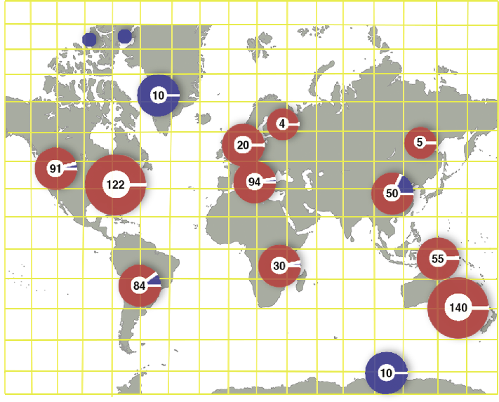
Figure 1: The Global Charcoal Database core locations (red, Daniau et al. 2012) and ice core sites to bedrock (blue) by geographic region. The numbers are the totals of both proxy records per location. The grid is a schematic representation of the ability of climate models to integrate multiple parameters over wide spatial scales and across areas where proxy data do not exist. |
Fires are an integral aspect of the Earth System, affecting climate through the release of aerosols and greenhouse gases, altering natural vegetation patterns and land carbon storage, and transforming land use. Charcoal, ice core, and modeling communities have been addressing climate and fire interactions from different perspectives. Each community has historically used separate approaches. This difference can partly be attributed to proxy availability or the necessity to produce data for various audiences including fire control and time-slice climate reconstructions. This workshop aimed at facilitating interactions between the three communities. The key workshop goals were to:
(1) Determine the status of existing data from each group and analyze the strengths and weaknesses of each data type,
(2) Identify how we can present our data so that each community (charcoal, ice core and modeling) can best use the results to further improve understanding of fire-related processes,
(3) Highlight ways to integrate the data of each group.
The charcoal community has compiled the Global Charcoal Database (GCD; www.ncdc.noaa.gov/paleo/impd/gcd.html) to create regional reconstructions and analyses of fire activity during specific time slices. Charcoal records can offer detailed local information that is often used to produce fire danger indices or to aid in land management. There are extensive charcoal records covering North America, the Mediterranean, and Australia, while other areas such as central Russia and Africa have sparse records, due in part to the lack of lakes with suitable sediments. The growing collaboration among researchers who study the impacts of fire and climate over regional scales will allow for the inclusion of charcoal records from larger lakes, permitting a more detailed understanding of fire history, particularly in data-sparse regions.
Ice core reconstructions of past fire activity complement charcoal studies because multiple parameters can be used to distinguish between fires from biomass fuel sources and those from fossil fuel emissions. Biomass burning tracers in ice cores with atmospheric residence times ranging from days to weeks include black carbon, elemental carbon, particulate organic carbon, monosaccharide anhydrides such as levoglucosan, organic acids, ammonium, nitrate and potassium, polycyclic aromatic hydrocarbons, and charcoal. Markers with an atmospheric residence time ranging from months to years tend to be hemispheric to global in scope. These ice core markers include carbon monoxide, δ18O of carbon monoxide, δ13C of methane, and non-methane hydrocarbons. The variety of tracers in ice cores allows the researcher to select markers based on a particular research goal, such as the production of high-resolution measurements or the unambiguous determination of past vegetation fires. Such reconstructions are steadily increasing, as new techniques demand smaller sample sizes. However, the multitude of ice core proxies and the novelty of many of these techniques currently create challenges for standardizing records into a compilation similar to the GCD.
Fire models are able to simulate fire-related processes at multiple spatial and temporal scales. Applied to past climates, the current generation of Earth System models is capable of providing regional reconstructions of changes in fuel load and moisture, biomass and burned area, and charcoal deposition. Atmospheric transport models are routinely used to estimate backward trajectories of aerosol particles and trace gases and to identify source and sink regions. Future work includes simulating the transport of tropospheric ozone or tracers such as organic biomarkers and black carbon, as well as a detailed comparison of simulated changes in burned area with charcoal and ice core proxies.
Workshop participants agreed that future research directions should focus on calibration studies for individual proxies, as well as between proxies. The workshop provided an opportunity to begin compiling and using an array of proxy data and model output to address major research questions in interdisciplinary fire science.
affiliations
1Department of Environmental Science, Informatics and Statistics, University of Venice, Italy; kehrwaldunive.it
2Institute for the Dynamics of Environmental Processes, Consiglio Nazionale delle Ricerche, Venice, Italy
3Department of Earth Sciences, Montana State University, Montana, USA
4Max Planck Institute for Meteorology, Hamburg, Germany
reference
Daniau A-L et al. (2012) Global Biogeochemical Cycles 26, doi:10.1029/2011GB004249
Bogdan P. Onac1, J.A. Dorale2 and J.J. Fornós3
NSF Workshop - Palma de Mallorca, Spain, 10-14 April 2012
Sea level history throughout the Quaternary shows a complex spatial and temporal pattern, and provides a globally averaged record of continental ice volume variations (Alley et al. 2005; Lambeck and Chappell 2001). Observations of this variability provide key constraints on the timing and amplitude of the forcing mechanisms that trigger the growth and decay of ice masses. With over a third of the world’s population living near coastlines, understanding the history and future impacts of global sea level change ranks as a top priority in the Earth sciences.
 |
|
Figure 1: Schematic cross-section through a coastal cave in Mallorca showing multiple levels of phreatic overgrowth on speleothems. Past sea water levels (long dashed lines) left clear encrustation marks on existing speleothems or along the cave walls (shown in yellow). Figure modified after Tuccimei et al. (2012). |
As uncertainties are inherent to the methodologies and settings of all sea level reconstructions, there is a continued need for additional, independent sources of sea level data that may provide unique insights and crosschecks to the existing framework of former eustatic changes in sea level. The coastal caves of Mallorca with their unique speleothem encrustations (Fig. 1) provide one such source of additional sea level data (Tuccimei et al. 2012), which can be used to precisely document the elevation and timing of various sea level stands in the western Mediterranean region with sub-meter resolution (Dorale et al. 2010). The western Mediterranean was chosen as the workshop site so that participants (especially those working with corals, ice, or models) could visit the coastal caves of Mallorca and acquaint themselves with the setting of this promising approaches (Fig. 1).
The purpose of the workshop was to bring together an international group of researchers to discuss and promote opportunities for collaboration on the topics of sea level data acquisition, calibration, and modeling. The meeting attracted 43 participants from nine countries, including 15 students and early career scientists. The workshop focused on the interpretation of sea level changes during marine isotope stage 5 (MIS 5) and the onset of MIS 4.
The event was organized into three distinct sections: two days of presentations (both oral and poster), two days of field trips, and a half-day round table discussion that concluded the meeting and explored directions for future research. The first section included 20 oral presentations, of which six were invited keynotes, and nine were posters. The speakers covered a wide spectrum of problems pertinent to sea level changes, including detailed studies of reef and marine terraces, submerged speleothems, marine notches, marine sediment sequences, phreatic overgrowth on speleothems, flank margin caves, cave minerals, timing of MIS 5, Quaternary fauna, and advanced sea level modeling studies. Sea level modeling was a major focus of discussion during the round table, which tackled the following topics: (1) ways of reconciling controversial MIS 5a data sets from sea level fields around the world, (2) the use of glacio-hydro-isostasy modeling to address the issue above, (3) challenges in addressing past sea level positions and how the community should bridge the gap between field observation and models, and (4) observational and modeling constraints on sea level rise/fall and ice extent/volume.
Finally, the workshop highlighted the interactions among researchers at various stages of their careers, from well-established scientists to junior faculty members, with particular emphasis on the participation of post-doctoral, undergraduate, and graduate students.
acknowledgements
The Organizing Committee would like to thank the U.S. NSF (OISE project #1022243), the Spanish Government's Ministerio de Economía y Competitividad/FEDER (project CGL2010-18616), PAGES, and USF Libraries for the generous financial and logistic support that made the workshop possible. Support by members of the Karst Research Group at the University of South Florida and students at the University of Balearic Islands were greatly appreciated.
affiliations
1Department of Geology, University of South Florida, Tampa, USA; bonacusf.edu
2Department of Geoscience, University of Iowa, USA
3Departament de Ciències de la Terra, Universitat de les Illes Balears, Palma, Spain
references
Alley RB, Clark PU, Huybrechts P, Joughin I (2005) Science 310: 456-460
Dorale JA et al. (2010) Science 327: 860-863
Lambeck K, Chappell J (2001) Science 29: 679-686
Tuccimei P et al. (2012) Quaternary International 262: 56-64
Andrea Dutton1, E.J. Stone2 and A. Carlson3
5th PALSEA Workshop - Madison, Wisconsin, USA, 6-8 June 2012
The 5th annual PAGES PALSEA Working Group workshop held in June 2012 was dedicated to understanding paleo constraints on future sea level rise. The main focus of this workshop was on ice sheet climate interactions and their implications for coastal engineering, although discussions also addressed a broader range of issues such as database efforts (A. Rovere, Columbia University, USA), ongoing challenges for modelers and observational scientists, and how and where these issues intersect. The workshop drew 39 participants, with strong international representation, bearing the hallmark of previous PALSEA workshops. A broad range of expertise was represented including climate and ice sheet modeling, glacial-isostatic modeling, and field-based techniques addressing prior ice sheet extent and relative sea level position – all the techniques needed to estimate future local sea level rise.
The sessions revolved around several themes, largely addressing ice sheet response and ice-climate interactions on a variety of timescales – from the early and late Holocene to previous interglacials as well as the Pliocene and the future.
 |
|
Figure 1: Surface mass balance in mm water equivalent (mm w. eq.) averaged spanning a 12-year period (2000-2011) according to mass accumulation rate simulations. Gray areas indicate the ablation area. Models from the last interglacial period discussed at the workshop identify the southwest region of Greenland as an area of significant retreat similar to present patterns of areas dominated by ablation versus accumulation. Figure from Box et al. (2012). |
In particular, among the variety of topics discussed, there was focus on the quantitative sources of additional water to the last interglacial sea level highstand. New analyses of Greenland Ice Sheet behavior during this time period were presented (Helsen et al. 2011; Stone et al. 2013; A. Quiquet, CNRS, France and D. Dahl-Jensen, University of Copenhagen, Denmark), in addition to a synthesis of Greenland Ice Sheet contributions from the past 20 years that generated in-depth discussion on the likely budget from Greenland and Antarctica. The geometry of the Greenland Ice Sheet during this time period was also discussed with different methodologies showing similar patterns of substantial loss of ice from the southwest (Fig. 1).
Another prominent topic was the deterministic versus stochastic nature of ice sheet response and the concept of ice sheet "weather" (M. Siddall, University of Bristol, UK). This led to a debate on the ability to use hazard analysis tools to assess the possible ice sheet contribution to sea level over the coming century based on the idea that outlet glaciers of ice sheets may not behave smoothly. Other discussions included assessments of the present (see Figure 1) and future behavior of the Greenland and Antarctic Ice Sheets from both a paleo and present modeling perspective (P. Applegate, Stockholm University, Sweden; P. Whitehouse, Durham University, UK; R. DeConto, University of Massachusetts, USA).
The mechanism of saddle collapse between ice domes in North America via a simple height-mass-balance feedback was proposed to explain rapid meltwater events during the last deglaciation (Gregoire et al. 2012). The applicability of this mechanism to other ice sheets of various sizes during different time periods was also discussed.
Data-oriented presentations focused on a wide range of questions and techniques on the Greenland and Antarctic Ice Sheets during the Holocene (J. Anderson, Rice University, USA; R. Hindmarsh, British Antarctic Survey, UK; Anders Carlson) and Pliocene (R. Ackert, Harvard University, USA), featuring summaries of field data for the 8.2-ka event (Törnqvist and Hijma, 2012) and of late Holocene ice sheet behavior (A. Long, Durham University, UK).
In addition to the scientific themes, workshop participants held discussions with Ben Strauss from Climate Central (climatecentral.org) to identify effective and appropriate public communication pathways on issues related to past sea level position and future sea level behavior.
On behalf of the workshop participants in Madison this year as well as those of previous PALSEA workshops, we would like to take this opportunity to thank Mark Siddall, Bill Thompson (Woods Hole Oceanographic Institution, USA), and Claire Waelbroeck (CNRS, France) for their leadership and vision over the past 5 years. PALSEA has been instrumental in bringing together diverse expertise to address common questions in the study of past ice sheet and sea level behavior with the goal of exploring what this knowledge brings to bear on future sea level change. We look forward to the ongoing multiplier effect of this collaboration throughout our community in the years to come, as Anders Carlson, Andrea Dutton, Antony Long and Glenn Milne (University of Ottawa, Canada) assume leadership.
acknowledgements
The organizers thank the following organizations for their support: PAGES, INQUA, the World Universities Network and the Department of Geoscience at the University of Wisconsin.
affiliations
1Department of Geological Sciences, University of Florida, Gainesville, USA; aduttonufl.edu
2School of Geographical Sciences, University of Bristol, UK
3Department of Geoscience, University of Wisconsin, Madison, USA
references
Box JE et al. (2012) The Cryosphere 6: 821-839
Gregoire LJ, Payne AJ , Valdes PJ (2012) Nature 487: 219-222
Helsen MM et al. (2011) American Geophysical Union, Fall Meeting 2011, abstract #C53C-0685
Stone E, Lunt DJ, Annan JD, Hargreaves JC (2012) Climate of the Past 9: 621-639