PAGES Magazine articles

Henning Thing

The European Union-funded Past4Future project aims at improving our knowledge of the climate system and the occurrence of abrupt climate changes during the last two interglacials, thereby paving the road for reducing the uncertainties in predicting future climate. The outcome of the project will eventually be globally disseminated and so far we have focused on the best way to communicate our results with citizens and policy-makers of the European Union.

For this purpose, we have (1) identified Past4Future stakeholders, (2) established a dialogue with them, using an online questionnaire, and (3) produced an assessment of their formulated needs and opinions. The online form presented 14 questions with a total of 78 multiple-choice options for answers as well as additional fields for entering detailed information. It took 10 to 12 minutes to complete the questionnaire.

Past4Future Stakeholders

We defined a Past4Future stakeholder as follows: an organization, a government agency, a commercial company or a community that has a direct or indirect stake in future climate change because it impacts its activities positively or negatively at a local, regional or global scale.

The aim was to receive feedback from at least 20 stakeholders. We identified and approached a total of 141 potential participants in very diverse positions, representing 22 European Union countries, Norway and the USA. The stakeholders were all contacted individually via targeted emails and friendly reminders. Unfortunately, we received feedback from only a few stakeholders: 18 people responded, but only 13 actually completed the questionnaire. Therefore, the opinions and comments expressed by the stakeholders in the review are based on these 13 feedbacks. A response rate of 9% illustrates how difficult it is to get the attention of the stakeholders although they have been individually approached and tended to. Our method obviously has not been successful; a personal face-to-face briefing with each stakeholder immediately before a paper-based questionnaire was scheduled would likely have produced a much higher response rate.

From the 13 stakeholders, seven come from the public sector (including politician, consultant, agency advisor), three are active in the private sector (e.g. consultant, media) and three are in the field of academia. Around half of the stakeholders operate in the strategic sphere, 30% conduct research and about 15% are in education fields.

Interests and opinions of the Past4Future stakeholders

However small the sample size is, the answers to the questionnaire form the foundation for assessing how to best present and disseminate the results and conclusions of the Past4Future project. This assessment is a first step to help the project partners to appraise stakeholders’ interests and needs, the communication pitfalls and the recommended ways in which project activities and results must be communicated widely to the science community, among policy-makers, other stakeholders, and to citizens of Europe and beyond.

Here are the main outcomes gathered from the 13 stakeholders:

Figure 1: An excerpt from the stakeholder survey: Feedback to the question "In which contexts do you use projections about future climate change?” Stakeholders were allowed to select multiple answers since they can use future climate change projections in more than one context.

Firstly, we consider their views on climate change projections: (1) These projections are most often used in a scientific context but stakeholders active in the public sector also use the projections for policy development (Fig. 1). (2) It is important for the stakeholders to know the exact information source, the assumptions made and the associated uncertainties. Stakeholders require projections on climate change risks to be founded in peer-reviewed sources or other sources of high credibility.

Secondly, their main scientific interests are in: (1) the anthropogenic increase of atmospheric greenhouse gas concentrations and (2) air and ocean temperature changes as well as sea level changes. The stakeholders are less interested in changes caused by solar and volcanic activity.

Thirdly, we consider their views on how to deliver the Past4Future project results (Fig. 2): (1) A personal briefing is preferred as the most useful method, supplemented by targeted information via email and website. (2) Press releases as well as written articles and conference presentations are considered useful means of delivering project results and conclusions. (3) Glossy brochures are deemed a waste of resources. In addition, most stakeholders estimate that information should be updated regularly.

Figure 2: An excerpt from the stakeholder survey: feedback to the question “How useful to you are the following methods of information delivery?” 11 of the 13 stakeholders responded to whether they found the different methods of delivery very useful, useful or not useful. The remaining two stakeholders provided written feedback.

Finally, in terms of the content, results should be delivered with an associated uncertainty. The stakeholder preference for this is an uncertainty that is expressed in “IPCC style” as they understand this concept. Again, they insist on the need to know the sources of uncertainty in the climate change projections.

Outlook

The delivery of Past4Future results into policy forums cannot be assumed and must be approached in a proactive manner. We will use forms, means and modes that will target the European perspective and impact our stakeholders. This will be achieved through various communicative products (including personal briefings, conference presentations, science journals, press releases, and public addresses) during the next two years, thereby enhancing Europe's ability to act timely and prudently while facing the challenges of the future climate.

affiliation

Centre for Ice and Climate, Niels Bohr Institute, University of Copenhagen; thinggfy.ku.dk

Sophie Verheyden1 and Dominique Genty2

We provide insights on speleothem sampling and describe the fieldwork involved in the retrieval campaigns of two calcite speleothems in the framework of the Past4Future project.

During the last decade, speleothem studies have enhanced our understanding of the evolution of continental climate thanks to the acquisition of high-resolution well-dated time-series (Cruz et al. 2005; Drysdale et al. 2009; Fleitmann et al. 2009; Genty et al. 2003; Genty et al. this issue; Wang et al. 2008). Speleothems can be precisely dated to up to 600 ka BP with the Uranium-Thorium method and potentially even further back in time if datable with the Uranium-Lead method.

Preparing for speleothem retrieval

Access to a cave for sampling is generally the result of long collaborations and much investment of time in order to build a trusting relationship with local cavers, cave owners, and cave managers. Also, speleothem sampling raises ethical issues related to their environmental, esthetical, and economic (touristic) significance. For this reason, sampling is usually conducted with respect to the few existing codes of ethics that provide specific guidelines for scientific work (UIS 1997, 2001; SSS-SGH 2004) (see FFS 2005 for an overview of the existing codes of ethics). Since the number of speleothem studies - and thus sampling - are rapidly increasing (Fleitmann and Spötl 2008), an enhanced exchange of already sampled speleothems through published literature or via internationally referenced museum collections is increasingly needed. This will help minimize the impact of speleothem research on cave environments.

To select the most appropriate speleothems to sample, cave monitoring (e.g. Genty 2008; Mattey et al. 2008; Verheyden et al. 2008) and preliminary dating is performed (Spötl and Mattey 2012). These first steps provide basic information on both the climatic response and growth period enclosed in the selected sample before its removal from the cave. Ongoing technical developments using portable in-situ imagery (Favalli et al. 2011; Hajri et al. 2009) and in-situ chemical analyses (Cuñat et al. 2005; Dandurand et al. 2011) will provide, in the future, information on the Uranium content and internal structure of speleothems, ensuring that scientists select the most appropriate in-situ samples without the need for preliminary laboratory work.

Retrieving speleothems

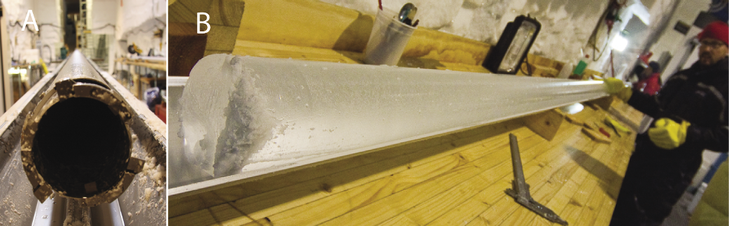
Figure 1: Speleothem samples taken in the framework of the Past4Future project. A) Core drilling of the RSM 17 stalagmite in the Remouchamps Cave, Belgium. The photo shows the drilling device used and the base of the stalagmite. B) Retrieval of a speleothem core. C) The stalagmite taken from Clamouse Cave, France. Photos: E. Zaremba, S. Verheyden, and D. Genty.

In the framework of the Past4Future project, scientists have collected new speleothem data covering the last interglacial period (LIG) and the penultimate deglaciation (Termination II). Among the new samples is RSM17, a broken stalagmite approximately 3-m-long and 1-m in diameter, from the Remouchamps Cave in southeast Belgium (BiSpEem project, Belspo 2012-2016). Preliminary Uranium-series dates indicate that the stalagmite was deposited between 126 [-11, +14] and 95.3 [-8, +9] ka BP with an overall growth-rate of 0.1 mm yr1 (Gewelt 1985). A team of seven people cored the stalagmite in May 2012. Since the stalagmite is located in a section of the cave open to tourists and close to the underground river, electricity and cooling water were available, facilitating the operation. However, the drilling was often interrupted by tourist visits. After six hours, 11 cores of ~30-cm -long and 8-cm-diameter were retrieved from the stalagmite (Fig. 1A-B). Sub-samples are currently at the University of Minnesota waiting to be Uranium dated.

In June 2012, a ~1.4-m-long and ~10-cm in diameter stalagmite was found broken on the floor of the Clamouse Cave (southern France), where other spelethems have already been sampled (McMillan et al. 2005; Plagnes et al. 2002; Quinif 1992) (Fig. 1C). The stalagmite was removed from the cave and ongoing dating is now needed to confirm that this stalagmite covers the LIG time period. The southern part of France benefits from optimal climate conditions enabling continuous speleothem growth during Termination periods, while speleothem growth further north generally only starts when full interglacial conditions are present.

Such a thin “take-away” stalagmite is ideal for studying the entire section, while drilled cores such as those from the Remouchamps Cave only reveal part of the internal section of the stalagmite. However, core drilling provides the possibility of sampling large stalagmites and flowstones. Importantly, drilling provides a unique opportunity to sample with minimal impact on the cave environment (Spötl and Mattey 2012).

Outlook

The speleothems sampled in the Remouchamps and Clamouse Caves in the framework of the Past4Future project are currently being analyzed. They will provide new chronological constraints on the onset of the LIG time period. They will also complement the existing speleothem dataset compiled by Genty et al. (this issue) with the aim of improving our understanding of the continental climate variability in Western Europe during Termination II and the LIG.

affiliations

1Geological Survey, Royal Belgian Institute of Natural Sciences, Belgium; sophie.verheydennaturalsciences.be

2Laboratoire des Sciences du Climat et de l’Environnement, CEA Saclay, Gif-sur-Yvette, France

acknowledgements

We thank the Remouchamps cave owners and managers, Y. Quinif, C. Ek, M. Gewelt, S. Delaby, cavers, Nicole Dubois and her team.

selected references

Full reference list online under: pastglobalchanges.org/products/newsletters/ref2013_1.pdf

BiSpEem Project – Belspo (2012 2016). Available at: www.naturalsciences.be/geology/research/environment/bispeem

Drysdale, RN et al. (2009) Science 325: 1527-1531

Spötl C, Mattey D (2012) Journal of Speleology 41: 29-34

UIS (1997) Available at: http://www.uis-speleo.org

Wang Y et al. (2008) Nature 451: 1090-1093

Jørgen P. Steffensen

We summarize the different approaches and logistical requirements for completing an ice core drilling. We also present the recent North Greenland Eemian Ice Drilling (NEEM) international project.

Ice cores are drilled in glaciers and on ice sheets on all of Earth’s continents. Whilst mountain glacier “shallow” ice core drilling reaches depths of ~300 m, “deep” drilling of several kilometers can be achieved on the Greenland and Antarctic ice sheets.

Drilling an ice core

Specialized drills are used to drill ice cores. They range in length from 3.5 m to 15 m. The devices hang on a steel cable with electrical wires inside allowing remote control from the surface. The cable runs from a winch over a top wheel on a vertical tower during drilling. Ice core drills can be either electromechanical or thermal.

Figure 1: Drilling an ice core. A) The drill head of the NEEM drill (photo: J.P. Steffensen). B) A freshly drilled 3.5-m ice core section at NEEM (Photo: T. Burton).

An electromechanical drill is simply a rotating pipe (core tube) with cutters at the head (Fig. 1A). During rotation, the cutters incise a circle around the ice to be cored until the core tube is filled with ice. The cuttings (also referred to as ice chips) are transported to a chip chamber in the drill. Rotation of the drill head is achieved by anchoring the motor section to the wall of the borehole with knife springs that allow sliding up and down but prevent any rotation. When the drill tube is full, the ice core is broken by a pull in the cable. Several barbs inside the core tube grab the core and break it. The drill is subsequently hoisted to the surface and in the case of most intermediate and deep-sized drills the drill and tower are tilted horizontally for easy removal of the core.

In the thermal drill, a ring-shaped heating element melts a circle around the ice to be cored and the melt water is stored in a tank in the drill.

Ice cores have typical diameters of 75 mm, 98 mm or 123 mm. They are usually retrieved in sections that are 1 m to as much as 4 m in length (Fig. 1B). As glacier ice deforms under pressure, it is necessary to fill the borehole with a drilling fluid for depths below 400 m to compensate for the increasing hydrostatic pressure of the surrounding ice with depth. This drilling fluid has a density slightly above the density of the glacier ice (920 kg m3) and thus prevents plastic deformation of the borehole and constriction of its width.

The logistics of ice core field camps

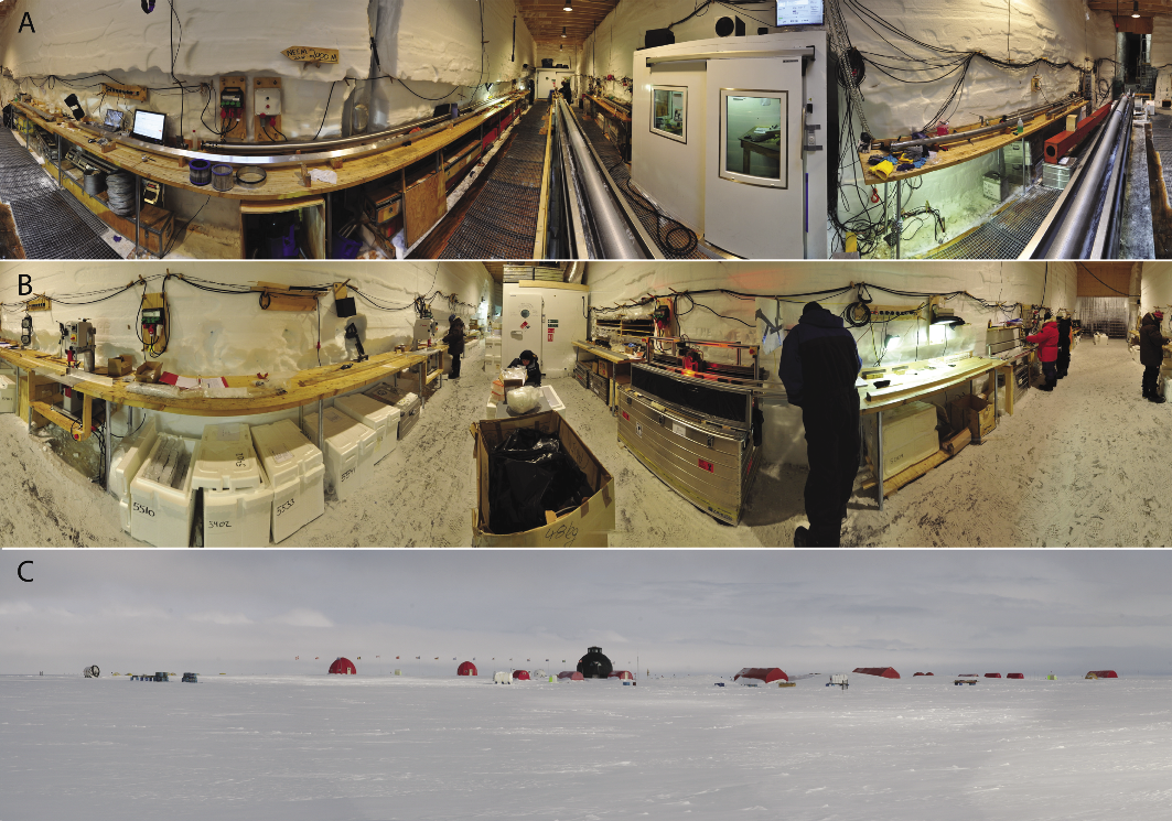
Figure 2: The NEEM ice coring project field camp. A) 360° view of the NEEM drill trench, 7 m below the surface (photo: M. Leonhardt and J.P. Steffensen). B) A 360° view of the NEEM science trench, 7 m below the surface (photo: M. Leonhardt and J.P. Steffensen). C) Panoramic view of the NEEM camp in the 2010 field season (Photo: J.P. Steffensen).

A “shallow” drilling for a 100-m-deep ice core can be performed on open snow as the drilling only takes a day or so. However, “intermediate” drilling to several hundred meters in depth may take weeks, and this is normally done in the shelter of a tent or in a covered snow trench (Fig. 2A). “Deep” drilling to more than one kilometer depth take many months and span several summer field seasons. In this case substantial infrastructure, such as a drill shelter, drill fluid supply and handling, electrical installations, campsite facilities, and organized transportation are needed.

The logistics involved in setting up and running a deep ice coring camp are considerable and costly (e.g. the total cost of the NEEM field activities was 7.4 million euros) and so far only 11 cores deeper than 1.5 km have been drilled worldwide. A substantial part of the costs occur from transportation, either over land by tractor train or, in the case of the NEEM project, by ski-equipped LC-130 Hercules air planes. In the past two logistical philosophies have been used:

• One can limit the scientific analyses in the field to an absolute minimum, which in principle reduces the expensive manpower required for this task. The ice cores are then cut and analyzed in cold rooms back home;

• One can do as many analyses in the field as possible, taking advantage of nature’s own clean “cold room” in an excavated science trench (Fig. 2B). This approach requires more manpower in the field; the advantages, though, are that scientists can work on the fresh core and that data are available at the end of the field campaign.

The key to a successful ice core drilling is the retrieval and documentation of an unbroken ice core, i.e. the top and bottom of an ice core section have to match up with the previous and subsequent cored sections. The core length (depth) must also be assigned with millimeter precision.

Drilling an ice core

The NEEM project (2007-2012) is the result of collaboration between 14 international partners and was initiated as an International Polar Year project. The strategy chosen was to perform as many analyses as possible on site.

Typical NEEM field season began May 1st and ended August 15th. A brief synopsis outlines the highlights from each field season during the project:

• 2007: The project team reached the NEEM ice core drilling site (77°N, 51°W, 2480 m above sea level) by tractor train from the former NGRIP ice core site some 365 km away.

• 2008: The team constructed the camp consisting of a four-level geodesic dome, two garage tents, a roofed drill trench and roofed science trench, a powerhouse and six tent buildings (Fig. 2C). The first 110 m of ice were drilled using a mobile “shallow” drill and the “deep” drill was installed in the drill trench.

• 2009 and 2010: The team completed the ice core drilling and ice core scientific processing. The first ice core with material from the bedrock was drilled in July 2010 at 2535 m depth. During these two seasons the camp population was around 35.

• 2011 and 2012: Special rock drill extensions were mounted on the drill and several meters of debris-laden ice from the base of the ice sheet were drilled. The NEEM camp was deconstructed in July and August 2012. Most of the camp infrastructure, including the geodesic dome, was designed to be stored on heavy sleds, ready to be towed to a future drilling site.

The drilling of the NEEM ice core was carried out by two shifts of two drillers and one mechanic with ~30 m of ice drilled per day. An average of 15 scientists were in the science trench to process the drilled ice with the work organized as an assembly line (Fig. 2B). Typical activities in the science trench consisted of documenting and cutting the cores into sections of 55 cm and performing a large range of measurements such as the Di-Electric Properties (DEP) and electrical conductivity of the ice (solid ice Electrical Conductivity Method, ECM). Thin sections of ice were also prepared to define the physical properties of the ice and volcanic tephra layers were sampled. In addition, we also conducted on-line Continuous Flow Analysis of the ice for dust, Na+, Cl-, SO42-, NO3-, NH4+, liquid conductivity, black carbon, formaldehyde, peroxide and Ca2+. For the first time, water isotope measurements by laser spectrometry and on-line measurements of gas concentrations by laser spectroscopy (CH4; see Blunier et al. this issue) were coupled with the main on-line system. The remaining ice core sections (such as those set aside for discrete gas concentration and water isotopes measurements) were then packed in insulated boxes and shipped to cold rooms in Copenhagen for storage.

More than 270 individuals spent a total of 12,520 man-days at NEEM. These persons consisted of 51% young scientists, 21% senior scientists, 20% logistics and 8% related to associated projects. In this way NEEM has not only been a project fulfilling a scientific objective to retrieve last interglacial ice (NEEM community members 2013; Dahl-Jensen this issue) but it has also been a unique opportunity for young scientists to gain fieldwork experience in the high Artic. For many of them, a stay at NEEM has laid the foundation for future successful international collaborations in ice core science.

affiliation

Centre for Ice and Climate, Niels Bohr Institute, University of Copenhagen; jpsgfy.ku.dk

reference

NEEM community members (2013) Nature 493: 489-494

Emma J. Stone1, P. Bakker2, S. Charbit3, S.P. Ritz4 and V. Varmav5

We describe climate modeling in a paleoclimatic context by highlighting the types of models used, the logistics involved and the issues that inherently arise from simulating the climate system on long timescales.

In contrast to "data paleoclimatologists" who encounter experimental challenges, and challenges linked to archive sampling and working in remote and/or difficult environments (e.g. Gersonde and Seidenkrantz; Steffensen; Verheyden and Genty, this issue) we give a perspective on the challenges encountered by the "computer modeling paleoclimatologist".

Simulating the physical interactions between atmosphere, ocean, biosphere, and cryosphere to explain climate dynamics is achieved through a large range of computer tools, from simple box models to complex three-dimensional (3D) fully coupled atmosphere-ocean general circulation models (GCMs) (see Box 1 for some examples).

Investigating the climate forcing and feedbacks that occurred during the past requires performing simulations on the order of thousands to tens of thousands of model years and due to computational time this is not easily achievable with a GCM. Therefore, compromises are required in terms of model resolution, complexity, number of Earth system components and the timescale of the simulation.

A suite of models referred to as Earth Models of Intermediate Complexity (EMICs) can effectively bridge the gap between computationally intensive GCMs and the box models (Claussen et al. 2002). These EMICs enable one to efficiently perform large ensembles and multi-millennial simulations whilst still retaining much of the behavior of a higher complexity model (e.g. Menviel et al. 2012; Ritz et al. 2011; Robinson et al. 2011). Although computing advancements have allowed transient climate experiments to be realized on long timescales, performing snapshot simulations with EMICs or GCMs is still frequent and useful (see Lunt et al. 2012).

Climate modeling by Past4Future

Within the Past4Future project numerous questions are addressed by modelers such as the sensitivity of climate to enhanced freshwater forcing, ice sheet changes and variations in solar and volcanic activity, using a range of EMICs and GCMs. Here, we highlight the implementation of multi-millennial transient simulations for the last interglacial period which include changes in astronomical and/or greenhouse gas concentrations (see Stone et al. this issue) using five climate models of varying degrees of complexity (see Box 1): CLIMBER-2 is a zonally-averaged model that permits basin-wide analysis, Bern3D includes a 3D ocean but a simple 2D atmosphere, LOVECLIM is of higher resolution (see Box 1), includes a low resolution GCM ocean but a simple three-layer dynamical atmosphere, FAMOUS is a low-resolution version of the UK Meteorological Office GCM (Gordon et al. 2000), and CCSM3 includes a fully dynamic atmosphere with the ability to be run at different resolutions (in this example the lowest resolution is used).

Although EMICs allow long time integrations to be easily realized, they parameterize a large number of processes (e.g. winds are fixed in Bern3D). The two GCMs, FAMOUS and CCSM3, have the advantage of including less parameterizations than the EMICs but they take months to run and generate large amounts of data. For instance, EMICs such as CLIMBER-2 and Bern3D have been able to simulate more than 800 ka in a few weeks. This is currently not achievable by models such as FAMOUS and CCSM3, which take several months to simulate only 10 ka.

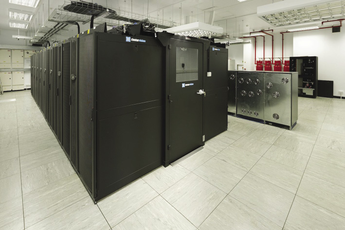
Figure 1: The machine room hosting the BlueCrystal supercomputer located in the Advanced Computing Research Centre (www.acrc.bris.ac.uk), University of Bristol (UK). Photo: Timo Kunkel.

Not only should the computational time be considered but also the ability to actually run the model code on a computer in terms of the power and the financial expense involved. Typically, climate models are written in numerically efficient computing code (e.g. FORTRAN), which can be implemented on a local desktop computer, as is the case for the EMICs given in Box 1. Otherwise, computationally intensive codes are run using high performance computing facilities such as the German HLRN supercomputer (used by CCSM3) or the "BlueCrystal" cluster at the University of Bristol (used by FAMOUS), which has the ability to carry out at least 37 trillion calculations a second (Fig. 1). These supercomputers are inherently expensive to implement, e.g. the BlueCrystal facility initially cost seven million pounds, with ongoing developments, and continuous maintenance incurring future costs. 

Maintaining and managing a climate model

Most model code is maintained centrally and in many cases can be downloaded freely by everyone. For example, the National Centre for Atmospheric Science looks after the FAMOUS model code in the United Kingdom and CCSM3 is maintained by the National Center for Atmospheric Research in the USA. Modelers from remote locations can submit new code but this needs to be peer-reviewed before being implemented into the next model version.

The EMIC models given in Box 1 comprise tens of thousands of lines of code while the GCMs contain more than half a million lines (see Easterbrook (2009) for details on the UK Meteorological Office model). Many individuals are involved in ongoing code modification and development, so version control is required to ensure errors are not inadvertently inserted. Good code development is also needed to ensure that any updates include clear and concise comments for users.

The technological development of increasing computer power, allowing climate researchers to run these multi-millennial simulations, large ensembles and GCM experiments, has presented a challenge with regard to what data should be written out and how it should be securely stored. The efficiency of some models such as CLIMBER-2, Bern3D and to an extent LOVECLIM, allows experiments to be repeated if more variables and different temporal resolutions (e.g. daily, monthly etc.) are required. This is not easily achievable with models such as FAMOUS and CCSM3. As such, careful decisions on what output would be useful are needed, not only for answering current research questions but also for long term future analyses, before the experiments are implemented.

The size of the output generated by the models in Box 1 varies greatly for a 10 ka simulation (depending on spatial and temporal resolution) from 400 MB to 6 TB. Normally, a sub-set of this data is stored on a storage facility that guarantees longevity and is ideally freely accessible. For example, the PANGAEA database (Data Publisher for Earth and Environmental Science; www.pangaea.de) is not only used for the secure storage of paleodata but also paleoclimate model results.

Closing remarks

The choice of a climate model has to be carefully considered in terms of included processes, the required spatial resolution, computational time and cost, the ability to obtain and run the model code and the storage space required for the model data. Although models are an incomplete representation of the Earth System, the advances in model development and computing technology over the last few decades have allowed researchers to consider more complex physical processes including a better understanding and consideration of the uncertainty in their model predictions (Hargreaves 2010). In the context of paleoclimatology this has greatly improved our understanding of the processes and feedbacks in the climate system.

Camilla S. Andresen1, F. Straneo2, M.H. Ribergaard3, A.A. Bjørk4, A. Kuijpers1 and K.H. Kjær4

Ice-rafted debris in fjord sediment cores provides information about outlet glacier activity beyond the instrumental time period. It tells us that the Helheim Glacier, Greenland’s third most productive glacier, responds rapidly to short-term (3 to 10 years) climate changes.

Sea-level rise is one of the major socio-economic concerns associated with global warming, since millions of people live within coastal floodplains that are situated less than 1 m above present sea-level. The latest IPCC report suggested a sea-level rise of 0.18 to 0.59 m within the next 100 years (IPCC 2007), but emphasized that the contribution from outlet glaciers is the largest source of uncertainty. Since then, several studies (see SWIPA 2011 for references) have suggested that the contribution from outlet glaciers could be +1 m or more.

Figure 1: (A) Main currents in the North Atlantic Ocean (Straneo et al. 2012) and location of Helheim Glacier (HG), Kangerdlugssuaq Glacier (KG) and Jakobshavn Isbrae (JI), (B) Helheim Glacier and Sermilik Fjord with position of the three cores (yellow dots) taken from water depths 500-600 m (bathymetry from Schjøth et al. 2012 and figure from Andresen et al. 2012) and (C) frontal variation in Helheim Glacier margin position from 1933 to 2010 grouped into time frames characterized by similar frontal behavior (from Andresen et al. 2012).

The concern about unexpected glacier dynamical behavior was highlighted when the three largest outlet glaciers in Greenland were observed to suddenly increase their discharge at the onset of this century. Specifically, Jakobshavn Glacier in west Greenland, Kangerdlugssuaq Glacier and Helheim Glacier, both in Southeast Greenland, accelerated, thinned and retreated between 2000 and 2005 (Fig. 1A, Rignot & Kanagaratnam 2006; Van den Broeke et al. 2009). In the case of Jakobshavn Glacier, researchers proposed that the acceleration was triggered by a warming of the subsurface ocean currents off West Greenland (Holland et al. 2008) consistent with the mid-1990s warming of the North Atlantic subpolar gyre, which feeds the waters off West Greenland via the Irminger Current (Buch et al. 2004; Holliday et al. 2008; Stein 2005). The ocean warming, in turn, was attributed to a shift from a positive to a negative North Atlantic Oscillation (NAO; Hurrell 2001) phase and additional changes in the low-pressure systems causing a westerly movement of the subpolar frontal system (Flatau et al. 2003; Hatun et al. 2005). The westward spreading of the warm subpolar waters contributed to a warming of the West Greenland continental shelf and an increase in the rate of submarine melting of the glacier front, thereby increasing iceberg calving rates and mass loss (Rignot et al. 2010).

This hypothesis of glacier melting caused partly by warm subsurface water penetration into the glacial fjords has also been suggested to explain the acceleration of outlet glaciers in Southeast Greenland (Christoffersen et al. 2011; Murray et al. 2010; Nick et al. 2009; Straneo et al. 2010). For example, Sermilik Fjord, where the Helheim Glacier terminates, is characterized by a thick layer of ~4°C warm Atlantic water of Irminger Current origin, underlying cold Polar water of glacial and Arctic origin (Fig. 1A; Straneo et al. 2010). However, as fjord water properties have only been monitored here since 2008, it has proven difficult to confirm such a causal relationship between oceanographic and glacier variability. Furthermore, relatively rapid mass changes of the Greenland ice sheet have only been estimated from satellite data since the early 1990s. Thus, a comprehensive understanding of the inter-annual to decadal variability of the ice sheet on longer timescales is lacking. Without longer records it is difficult to evaluate if the recent mass loss is an outstanding event or is part of a recurring phenomenon acting on inter-annual, decadal or centennial timescales, or a combination of both.

Reconstruction of Helheim Glacier calving variability

Figure 2: Comparison between the calving record and climate indices for Helheim Glacier (note the lack of some climate data during the 2nd World War). (A) Reconstructed calving record of Helheim Glacier from the three sediment cores (Thick lines are 3-year running mean data and thin lines are unfiltered data), (B) Helheim Glacier margin positions indicated relative to the 1993 position according to aerial and satellite images (color coding as in Fig.1C), (C) summer Tair from Cappelen (1995), (D) SST south of Iceland (Andresen et al. 2012), (E) Storis Index (northernmost multi-year sea ice extent observed off southwest Greenland) from Schmith and Hansen (2003) and updated for 2000-2007 in Andresen et al. (2012), (F) Shelf Index (Andresen et al. 2012) and (G) NAO data from www.cru.uea.ac.uk/cru/data/nao. (Note AW =Atlantic Water and PW= Polar Water). Figure modified from Andresen et al. (2012).

The link between climatic changes and outlet glacier variability was recently investigated in a study of past changes of Helheim Glacier going back 120 years, analyzing three marine sediment cores retrieved in Sermilik Fjord (Fig. 1B; Andresen et al. 2012). We reconstructed the calving variability based on the assumption that changes in the deposition of sand (ice-rafted debris) directly relate to changes in iceberg rafting from calving activity. The resulting record documents a series of calving events lasting 3 to 10 years (Fig. 2A). The use of the sand deposition as a recorder of the calving history of Helheim Glacier is supported by the agreement between the reconstructed calving changes and the changes in frontal position of the Helheim Glacier since 1933 as observed from satellite data and historical aerial photographs (Fig. 1C, Fig. 2A-B).

Exploring a link with climate

Increased air and ocean temperatures (both surface Polar water and subsurface Atlantic water) may increase glacier calving through a number of processes involving destabilization of the glacier margin (Motyka et al. 2011). Examples of such processes are ocean water undercutting and melting the submerged glacier margin, surface glacial melt water penetrating down the ice sheet, forming crevasses and promoting iceberg formation, or destabilization of the dense ice mélange (mixture) of icebergs and sea ice in front of the glacier margin (Amundson et al. 2010; Vieli and Nick 2011). To investigate potential links between climate variability and Helheim Glacier instability we compared the calving history with records of nearby oceanic and atmospheric variability (Fig. 2). Air temperature variability was taken from the observed summer temperatures at Tasiilaq (Fig. 2C). No long-term ocean measurements are available from Sermilik Fjord or the nearby shelf. Therfore, we used several indirect indicators for subsurface Atlantic water and surface Polar water: (1) Direct measurements of sea surface temperature (SST) from south of Iceland, where Atlantic water extends to the surface while flowing towards southeast Greenland and sliding underneath the East Greenland Current, were used as a measure of Atlantic water variability (Fig. 2D). (2) Changes in the Storis Index related to the amount of sea ice in the East Greenland Current, were used as a measure of Polar water variability (Fig. 2E). (3) Atlantic water and Polar water variability were combined into a so-called Shelf Index (Fig. 2F) assuming that the variability of waters on the shelf mostly reflects changes in the relative volume of these water masses: a positive Shelf Index indicates a thicker and warmer Atlantic water (at the expense of Polar water) and vice versa.

Finally, we compared the calving record with the wintertime NAO Index, which represents the dominant mode of atmospheric climatic variability in the North Atlantic region (Fig. 2G).

Rapid glacier response to climatic changes

We find that the calving variations are linked with synchronous changes in the source of Atlantic water and with local summer air temperature at multi-decadal timescales. Both these climate parameters reflect the Atlantic Multi-decadal Oscillation (Schlesinger and Ramankutty 1994) in this region. Therefore, we were unable to separate their respective impacts on the Helheim Glacier variability.

At sub-decadal timescales (3 to 10 years), calving peaks correlated with short-term episodes of positive Shelf index and negative NAO index. As previously mentioned a negative NAO phase is often associated with a warm subpolar gyre and increased penetration of Atlantic water on the shelf (Holland et al. 2008), but local wind and air temperatures as well as variability in both the Polar water and Atlantic water source regions also often co-vary with the NAO index on these timescales (Dickson et al. 2000).

The most important finding from this study is that the increase in calving activity observed at Helheim Glacier during the period 2000 to 2005 is only matched in magnitude by a calving event in the late 1930s (Fig. 2). These two episodes are distinct from other calving episodes in our record. This is because they are the only two events that occur during a time interval characterized by the coincidence of a positive (warm) AMO phase, exceptional (for the investigated time period) high summer temperatures, and low Polar water export. The NAO Index was also frequently negative in the late 1930s, though not markedly more negative than during many of the other calving episodes.

Summary

Our study of three sediment cores from the Sermilik Fjord shows that Helheim Glacier responds to changes in large-scale atmospheric and oceanic conditions on timescales as short as a few years. The magnitude of the increase in calving activity observed at Helheim Glacier from 2000 to 2005 is only comparable to a calving episode that occurred in the late 1930s. A comprehensive understanding of the timescales involved in glacier changes and of the influence of oceans and atmospheric variability is important, if we are to make reliable predictions of future glacier changes and associated sea-level rise in a warming world.

acknowledgements

This study has been financially supported by Geocenter Denmark and the SEDIMICE project, the Danish Council for Independent Research - Nature and Universe (Grant no. 09-064954/FNU), the Danish Agency for Science, Technology and Innovation as a part of the Greenland Climate Research Centre and NSF ARC 0909373.

The reconstructed Helheim glacier calving record can be downloaded from the Pangaea database.

affiliations

1Geological Survey of Denmark and Greenland, Department of Marine Geology and Glaciology, Denmark; csageus.dk

2Department of Physical Oceanography, Woods Hole Oceanographic Institution, USA

3Danish Meteorological Institute, Centre for Ocean and Ice, Denmark

4Centre for GeoGenetics, Natural History Museum, Denmark

selected references

Full reference list online under: pastglobalchanges.org/products/newsletters/ref2013_1.pdf

Andresen CS et al. (2012) Nature Geoscience 5: 37-41

Buch E, Pedersen SA and Ribergaard MH (2004) Journal of Northwest Atlantic Fishery Science 34: 13-28

Holland D et al. (2008) Nature Geoscience 1: 659-664

Schmith T and Hansen C (2003) Journal of Climate 16: 2782-2791

Straneo F et al. (2010) Nature Geoscience 3: 182-186

Aurélien Mairesse and Hugues Goosse

The data assimilation technique applied to paleoclimate studies is a promising method to highlight the compatibility or the incompatibility between (1) different climate proxies and (2) between climatic information inferred from the proxies and the physics of the climate system represented in models.

The combination of several climate proxies and/or the results from climate models enables us to reconstruct and understand past climate changes. When data and models are used together, the information inferred from the proxies often serves to validate the climate model results while the models allow exploration of the physical processes responsible for the recorded climatic changes. During the past decade, a new statistical tool called data assimilation has been used in paleoclimatology (Widmann et al. 2010). This tool allows us to build a reconstruction of past climate change which is both consistent with the climate computed by a model and that deduced from proxies.

First, we describe how this tool works when it is applied to the paleoclimate research field. Second, we describe a particular application of data assimilation, which can help to elucidate if the hypotheses proposed to explain proxy variations are compatible with the physics of a climate model. This is outlined with a mid-Holocene case study.

How does data assimilation work?

Figure 1: Inferred mid-Holocene surface temperature anomalies (°C) compared to a reference period (1000 to 1500 AD). Where there is more than one proxy record at the same location, the markers representing the proxies are slightly shifted for improved readability.

Data assimilation combines the physical laws included in a climate model with the climate information inferred from proxies to produce paleoclimatic reconstructions consistent with both. In our method, this is achieved using a procedure based on a particle filter with resampling (Dubinkina et al. 2011; see Fig. 1 from van Leeuwen 2009 for a graphical representation) applied to the three-dimensional Earth model of intermediate complexity, LOVECLIM (Goosse et al. 2010).

An ensemble of ~100 simulations, also referred to as particles or ensemble members, is initiated in parallel. At the beginning of this procedure, all of the particles are identical apart from slightly different initial conditions. Due to the chaotic nature of the climatic system each particle will evolve in a different way. After the first assimilation step (which is one year here but it can be any value greater than or equal to the model time resolution) the likelihood of each member of the ensemble is evaluated in order to determine how close the climate state of each particle is compared with the climate inferred from the proxy data. For each variable (e.g. surface air temperature and sea surface temperature; SST) the likelihood is a function of the difference between the values estimated from the proxy records and the values calculated by the climate model. This function is computed for all the locations and months for which paleodata is available. The particles that have the largest likelihood are retained (i.e. the particles whose climate states are the closest to the past climate reconstructed from the proxies). The other ensemble members are rejected. The remaining particles are resampled in order to keep a constant number of particles (i.e. ~100 in this example) and avoid a degenerative issue. We add a small perturbation to the members that have been sampled more than once for the next year of assimilation. The whole procedure is continually repeated until the final year of calculation (i.e. if we perform a 200-year simulation the procedure is repeated 200 times in this example).

The final climate reconstruction obtained by this method is consistent with the LOVECLIM physics, since the LOVECLIM climate model itself is used in the assimilation process. The reconstruction is also as consistent as possible with the climate derived from the proxy data. This is because the method only selects LOVECLIM results that are most compatible with the information inferred from all the climate proxies, for each time step of the simulated time period.

Our method has produced a reconstruction of surface temperature changes over the past millennium (e.g. Goosse et al. 2006, 2012). The data assimilation in those studies performed well since the LOVECLIM results were efficiently constrained to be close to the surface temperature signal recorded by continental data and, therefore, provided a consistent picture of the climate system during these particular time periods. Recently, we have applied this data assimilation method to the mid-Holocene climate.

Data assimilation applied to the mid-Holocene

A large number of surface air and SST reconstructions are available for the Holocene. A selection from more than 300 published records was performed with the following criteria: (1) each record must come from archives located between 20°N and 90°N and (2) each record must have a mean temporal resolution of at least 250 years for the period of interest (6.5 to 5.5 ka BP).

In accordance with these two principles and restricting selection to only publicly available data, we selected 47 records of surface air temperature and SST for the mid-Holocene. The resulting dataset is heterogeneous for the following reasons: (1) this climatic information was inferred from climate proxies preserved in marine, continental, and ice archives (Fig. 1), (2) for a given archive, different proxies have been used to infer the same type of information (e.g. SST reconstructions in marine cores based on alkenones, Mg/Ca ratio etc., Fig. 1) and (3) the proxies have been measured and interpreted in term of climate variations by different research groups.

We have performed the first mid-Holocene data assimilation with the selected dataset and the LOVECLIM model. For this 200-year snapshot experiment, the constraint provided by data assimilation is weak and the disagreement between the climate proxies and model results based on this data assimilation method is still large. For all the locations and the months for which proxy information is available, the LOVECLIM results with data assimilation are on average only 10% closer to the climate signal extracted from the proxies than with the LOVECLIM results produced without data assimilation. In other words, because of the heterogeneous nature of the proxy dataset, the simulations with data assimilation mainly highlight incompatibilities between the proxies and with the model physics rather than producing a shift of the model state that results in a better agreement with the proxy-based climatic reconstructions.

Incompatibilities between proxy and model

First, some variations observed in the climate reconstructions inferred from the proxies cannot be explained by LOVECLIM because they are related to phenomena occurring at a scale smaller than the model grid resolution. For example, this is the case with some SST reconstructions from marine cores retrieved in coastal margins such as the Tagus Estuary (Portugal) where Holocene SST variations are partly influenced by the Tagus River input (Rodrigues et al. 2009). Such a regional influence in this area is not represented in the LOVECLIM model.

Second, incompatibilities exist between reconstructions based on different types of proxies (see Fig. 1). Future work will aim at identifying these inconsistencies by performing additional experiments with data assimilation. We will run several ensemble simulations, each constrained by climate records from only one type of proxy at a time (e.g. pollens). Each set of simulations will enable the identification of the processes that could explain the recorded signal used according to the climate model physics. Subsequently, it will be also possible to analyze the results of these experiments at locations where other proxies, not selected to drive this set of simulations, are available. For instance, we will compare the results from an assimilation which includes only pollen data, with SSTs inferred from alkenones. This comparison could aid in deciphering whether the SST signal deduced from alkenones should be interpreted as an annual or a summer signal to improve the compatibility between the pollen and the alkenone-based climate records, according to the LOVECLIM physics. This procedure may lead to a tentative revised interpretation of the climate proxy. Even if this proves too challenging, the uncertainty in model-data comparison associated with incompatibilities between proxy-based reconstructions could at least be estimated.

Outlook

We highlight the potential use of the data assimilation method for paleoclimate studies. This method enables us to assess compatibilities and/or incompatibilities between different climate proxy records for the mid-Holocene time interval. In the future, we could use data assimilation to suggest a revised interpretation of the proxies in order to have a better consistency between different climate proxies and enable more accurate model-data comparisons.

affiliation

Georges Lemaître Centre for Earth and Climate Research, Earth and Life Institute, Université catholique de Louvain, Belgium; aurelien.mairesseuclouvain.be

selected references

Full reference list online under: pastglobalchanges.org/products/newsletters/ref2013_1.pdf

Dubinkina S et al. (2011) International Journal of Bifurcation and Chaos 21: 3611-3618

Goosse H et al. (2006) Climate Dynamics 27(2): 165-184

Goosse H et al. (2010) Geoscientific Model Development 3(2): 603-633

Goosse H et al. (2012) Global and Planetary Change 84-85: 35-47

van Leeuwen PJ (2009) Monthly Weather Review 137(12): 4089-4114

Natalie Kehrwald1, P. Zennaro1,2 and C. Barbante1,2

Fire impacts climate by changing atmospheric greenhouse gas concentrations, vegetation distributions, and surface albedo. We present a biomarker, levoglucosan, to reconstruct past fire activity from ice cores. This tracer allows us to investigate fire and climate interactions over glacial-interglacial cycles.

The devastating Waldo Canyon fire (North America) forced the evacuation of approximately 30,000 people from their homes in Colorado Springs during June 2012 (Fig. 1). The massive wildfires and associated heat wave that swept across Russia in 2010 were responsible for the deaths of over 55,000 people (Barriopedro et al. 2011), caused 15 billion US dollars in damages and were the result of both natural and anthropogenic climate change (Otto et al. 2012). This destruction demonstrates the importance of understanding the prospect of increased fire activity in a changing climate.

Interactions between climate and fire activity

The relative impact of climate change (including increased deadwood availability due to bark beetle infestations) and human activity on fires (including forest management and housing expansion) can differ between individual fires. Droughts tend to increase fire activity, provided that there is sufficient material to burn. Increased precipitation may also cause more vegetation growth and increase the area susceptible to burning as long as the precipitation remains low enough that it does not suppress fires. Regional fire activity, therefore, depends on a number of variables including temperature, fuel availability, and precipitation, but generally increasing global temperatures enhance global fire activity (Daniau et al. 2010; Power et al. 2008).

Fires in turn, influence climate by emitting greenhouse gases and aerosols into the atmosphere, and by affecting carbon sequestration in vegetation and soils. Deforestation fires alone have caused ~19% of the anthropogenic warming since preindustrial times (Bowman et al. 2009). Currently, total biomass burning releases up to 50% as much carbon dioxide into the atmosphere as does fossil fuel combustion (Bowman et al. 2009). The impact of biomass burning emissions on the global radiation balance and the carbon cycle, however, remains one of the least understood aspects of the climate system.

It is essential to determine the interactions between climate and fire activity through time in order to establish if humans are increasing susceptibility to fire in a warming climate. The last interglacial period (LIG, ~130-116 ka BP), represents a climate analogous to the present but without the impact of human activity. Ice core records from the LIG and present interglacial contain contemporaneous climate and fire proxies that allow a detailed assessment of fire activity in warming climates with and without anthropogenic influences.

Fire and climate records in ice cores

Researchers have developed many fire proxies in ice cores during the past decade. Tracers for biomass burning in ice cores with atmospheric residence times ranging from days to weeks include black carbon, particulate organic carbon, monosaccharide anhydrides, organic acids, diacids (oxalate, formate), major ions (ammonium and potassium), isotopes of carbon monoxide and methane, polycyclic aromatic hydrocarbons, and charcoal. In general, the shorter residence time tracers provide more regional records, while the longer residence time tracers can provide hemispheric to global records of biomass burning. Here, we discuss using monosaccharide anhydrides as fire tracers and their applicability to the present and past interglacials.

Figure 2: (A) Atmospheric transport of smoke plumes from the western Hudson Bay forest fire source to the study site (AGL = above ground level). (B) Multiple years of fire markers (ammonium, potassium, and oxalate) determined from a 6-m deep snow pit at Summit, Greenland. Note that the sodium concentration record, also shown, is one of the main tools to date the snow pit (peaks in sodium denote spring accumulation). (C) Comparison between oxalate and levoglucosan as biomass burning tracers in the upper section of the snow pit. The black arrows on (B) and (C) point to the same known Canadian fire event. Figure modified from Kehrwald et al. (2012).

Biomass burning injects monosaccharide anhydrides such as levoglucosan into the fine particle phase of smoke plumes. Levoglucosan is a specific tracer of fire activity as it is only derived from cellulose burning at temperatures greater than 300°C (Schkolnik and Rudich 2006; Simoneit 2002). Levoglucosan is injected into and travels through the atmosphere in smoke plumes before returning to the surface through wet and dry deposition (Fraser and Lakshmanan 2000; Stohl et al. 2007). We trace levoglucosan from a forest fire source to its deposition on glacier surfaces where it is preserved and does not appear to decompose in snow and firn layers (Fig. 2A; Kehrwald et al. 2012). Levoglucosan is unequivocally a cellulose degradation product (Simoneit 2002), while other biomass burning tracers archived in snow and ice cores may have multiple sources.

We investigated samples from a snow pit at the Summit camp in Greenland and combine levoglucosan records with other biomass burning proxy records to provide an analysis of past fire activity from 1987 to 1995 (Fig. 2B-C). We demonstrate that combining levoglucosan concentrations with other biomass burning proxies helps determine the relative contribution of fire versus other sources to total deposition. This is illustrated by an event that occurred between spring 1994 and spring 1995:

• The oxalate and levoglucosan peaks replicate the same known Canadian fire event (Fig. 2C). Although oxalate is a product of forest fire emissions (Legrand and DeAngelis 1996) it may also originate from vehicle emissions (Kawamura and Kaplan 1987).

• Ammonium concentrations in the snow pit also peak during the fire event, but the increased concentrations are distributed across a relatively wide depth range (Fig. 2B). Elevated concentrations of ammonium (Stohl et al. 2007) may reflect past fires, but atmospheric ammonium may also result from lightning, marine sources, soil processes, or agricultural activity (Hristov et al. 2011; Olivier et al. 2006).

• While potassium concentrations have been identified as a past fire activity proxy (Echalar et al. 1995) they do not reproduce the oxalate and levoglucosan peaks in our record (Fig. 2B). Potassium can be transported to glacier surfaces through sea salts and mineral aerosols (Laj et al. 1997). The differing transport paths and sources of levoglucosan and potassium are reflected in the snow pit concentrations. As a result, if the fire reconstruction from this snow pit were assessed solely from potassium concentrations, they would miss an important fire event.

The research team at the University of Venice has created high-resolution Holocene levoglucosan records from the NEEM and EPICA Dome C (EDC) ice cores and a late Holocene levoglucosan record from Kilimanjaro ice cores. This combination creates a pole-equator-pole transect of Holocene fire records. The Kilimanjaro ice fields are located near the largest savanna system in the world. Savanna and similar grassland fires produce the highest levoglucosan emission factors of various tested vegetation types (Engling et al. 2006) and Kilimanjaro may serve as reference site for high levoglucosan concentrations. NEEM and EDC are located farther away from levoglucosan sources than Kilimanjaro, but both of these polar locations archive a levoglucosan flux above the detection limit. Late Holocene NEEM levoglucosan concentrations correlate with synthesized charcoal records above 55°N, demonstrating the viability of using levoglucosan concentrations in ice cores as a biomass burning tracer over centennial to millennial timescales. This correlation between sedimentary charcoal and ice core records allows researchers to reconstruct fire histories over larger spatial scales.

The research team is currently determining LIG levoglucosan concentrations from NEEM and EDC ice cores to compare with the Holocene records. Initial tests are encouraging and demonstrate that the LIG ice contains detectable levoglucosan concentrations.

Outlook

Human activities including slash-and-burn farming, forest fires caused by human ignition, and wildfire suppression alter global fire activity. Anthropogenic activity also increases greenhouse gas concentrations, resulting in warming temperatures and possibly increased wildfires. Paleorecords demonstrate that global fire activity is higher during interglacials than during glacial periods in a purely natural system (Daniau et al. 2010). Imminent measurements of LIG levoglucosan concentrations will provide unique constraints on past fire activity in a warming climate with implications for fire activity in the current climate.

acknowledgements

The research leading to these results has received funding under grant agreement no 267696, (ERC-2010-AdG_20100224) ”EARLYhumanIMPACT. How long have humans been impacting the climate system?”

affiliations

1Department of Environmental Sciences, Informatics and Statistics, University of Venice, Italy; kehrwaldunive.it

2Institute for the Dynamics of Environmental Processes, Consiglio Nazionale delle Ricerche, Venice, Italy

selected references

Full reference list online under: pastglobalchanges.org/products/newsletters/ref2013_1.pdf

Bowman DMJS et al. (2009) Science 324: 481-484

Engling G et al. (2006) Atmospheric Environment 40: 299-311

Kehrwald N et al. (2012) Tellus B 64, doi: http://dx.doi.org/10.3402/tellusb.v64i0.18196

Schkolnik G, Rudich Y (2006) Analytical and Bioanalytical Chemistry 385: 26-33

Simoneit BRT (2002) Applied Geochemistry 17: 129-162

Valérie Masson-Delmotte1, E. Capron2, H. Goosse3, K. Pol2, M. Siddall4, L. Sime2, S. Bradley4 and B. Stenni5

New studies focusing on Antarctic climate variability during the current and earlier interglacial periods highlight the interplay between long-term climatic changes and climate variability in Antarctica, and enable the fingerprint of past changes in ice sheet topography to be investigated.

New findings have arisen in the framework of two ongoing European projects that aim at documenting and understanding past Antarctic climate variability. The ESF HOLOCLIP project focuses on Antarctic and marine records of the Holocene (~15-0 ka BP), while the Past4Future project aims at, among other things, improved spatial and temporal coverage of the last interglacial (LIG; ~129-118 ka BP) in water stable isotopes from Antarctic ice cores.

By combining both data and model results obtained during two interglacial periods, characterized by different orbital configuration and over a large range of timescales (from multi-decadal to orbital), we show how these studies contribute to assessing the mechanisms responsible for Antarctic climate variability, and how they inform on the fingerprint of changes in ice sheet topography.

The last millennium

Figure 1: Antarctic records of the present interglacial and the last interglacial periods. This panel shows temperature estimates simply based on the spatial isotope-temperature gradient (0.8‰ δ18O per °C) using (A) a stack of seven ice cores for the last millennium and using individual ice cores (Vostok, VK; Dome F, DF; EPICA Dronning Maud Land, EDML; EPICA Dome C, EDC; Talos Dome, TALDICE) and the mean signal extracted using the first principal component (EOF1) for (B) the present interglacial and (C) the LIG. Modeling studies have suggested that past changes in isotope-temperature relationships could lead to larger temperature changes than depicted here (e.g. Sime et al. 2009).

A good estimate of the magnitude and patterns of Antarctic temperature at a multi-decadal to centennial timescale during the last millennium is essential to understand the response of Antarctic climate to external forcings, and for assessing the ability of climate models to resolve the mechanisms at play (Goosse et al. 2012). Within HOLOCLIP, a composite of Antarctic temperature has been calculated by averaging temperature anomalies derived from seven ice core records (Fig. 1A). This simple method is supported by the coherency displayed between the average of the climate model results at the corresponding grid points, and the simulated average Antarctic temperature. Models and data rule out large (>0.5°C) preindustrial temperature variations during the last millennium, and show ~0.5°C warming since 1850 AD. Climate model simulations mainly attribute the multi-centennial cooling trend depicted from 1000 to 1850 AD to volcanic forcing for annual mean temperature, while orbital forcing controls seasonal trends. Ongoing work aims at improving the documentation of Holocene climate and sea ice variability by combining ice core water stable isotope (Fig. 1B) and aerosol records with information from deep-sea sediments and coastal records.

Interglacial climate: mean state and variability

Antarctic ice core records provide insight to a diversity of interglacial periods, characterized by different durations, intensities, and trends (Jouzel et al. 2007; Uemura et al. 2012). Within the Past4Future project, new high-resolution water stable isotope measurements have been performed in order to assess past changes in high-resolution variability. In central Antarctica, deposition and post-deposition processes such as precipitation intermittency and wind scouring limit the relevant temporal resolution to approximately 20 years. So far, a 45-year resolution has been achieved for Marine Isotopic Stage (MIS) 11 (~400 ka, Pol et al. 2011) chosen as an exceptionally long interglacial, and a 20-year resolution for the LIG (Pol et al. unpublished data), chosen as an exceptionally warm period.

In Antarctica, MIS 11 is marked by a multi-millennial-long increasing trend, which then decreases. High-resolution deuterium measurements have revealed increased sub-millennial climatic variability in the decreasing temperature phase. During the LIG (Fig. 1C), Antarctic temperature exhibits an early maximum, which corresponds to a bipolar seesaw with respect to Northern Hemisphere climate (Masson-Delmotte et al. 2010). It is followed by a multi-millennial scale plateau, then by a cooling into the glacial inception, punctuated by the onset of glacial millennial climatic variability, established at around 110 ka BP (Capron et al. 2012). Our unpublished high-resolution deuterium data point to minimum variance during the LIG "plateau", above Holocene levels and an increasing sub-millennial climatic variability at the end of the interglacial phase, as observed for MIS 11.

Tracking changes in the Antarctic ice sheet topography

Further investigation of the Antarctic climate during the LIG was achieved by comparing the records available from six East Antarctic ice cores with their Holocene data. In addition to the common features previously described and well captured in the EPICA Dome C ice core, the same regional differences are depicted during the current and LIG periods. Some earlier studies have shown that these differences can be attributed to precipitation intermittency (e.g. Sime et al. 2009). However, an alternative interpretation lies in different elevation histories due to the interplay between local ice thickness and isostatic adjustment.

The cause for peak Antarctic warmth during the LIG remains disputed. Astronomical forcing alone does not allow climate models to produce warmer than present day Antarctic temperatures. Therefore, other hypotheses such as the bipolar seesaw linked with large-scale ocean circulation perhaps along with the climate impacts of a collapse of the West Antarctic ice sheet (Holden et al. 2008), could explain the early Antarctic optimum. Recent studies have stressed that the Greenland ice sheet may have made only a limited contribution (about +2 m of equivalent sea level) to the LIG highstand, pointing to a significant contribution of the West and/or East Antarctic ice sheets to the estimated 6-to-10-m high stand (NEEM community members 2013; Dahl-Jensen et al. this issue).

Figure 2: Simulated impacts of changes in Antarctic ice thickness and isostatic adjustment. Circles indicate ice core sites (Vostok, VK; Dome F, DF; EPICA Dronning Maud Land, EDML; EPICA Dome C, EDC; Talos Dome, TALDICE; Taylor Dome, TD) and the solid black lines highlight the location of the edge of each ice sheet model used. (A) Predicted stable isotope trends (‰ kyr-1) driven by surface elevation changes only (not accounting for climatic impacts) resulting from a collapse of the WAIS (from 130 to 118 ka BP). Note that the dark red and orange colors represent ‰ kyr-1 values greater than the maximum (20) and minimum (-4) on the scale bar, respectively.(B) Difference in the predicted stable isotope trends (‰ kyr-1) between a reference LIG Antarctic ice sheet model (Bradley et al. 2012) and a model (Bradley et al. 2013) where a significant retreat of marine-based ice in the Wilkes and Aurora basins of the East Antarctic Ice Sheet (from 126 to 118 ka BP) has been simulated. Modified from Bradley et al. (2012) and Bradley et al. (2013).

At the intersection of Past4Future Work Packages focused on interglacial climate variability and ice sheet dynamics (e.g. Siddall et al. this issue), different Past4Future partners have started to explore if a fingerprint of past changes in the Antarctic ice loading could be detected as an elevation-driven temperature trend preserved in East Antarctic ice cores. A “treasure map” was produced, identifying potential drilling sites where a clear fingerprint of a West Antarctic ice sheet collapse could be identified (Bradley et al. 2012). These sites, unfortunately, do not coincide with existing ice core records (Fig. 2A). The same approach proved more successful for the Wilkes-Aurora Basin sector of the East Antarctic ice sheet, and preliminary results (Bradley et al. 2013), assuming a homogeneous climate history, suggest that differences between the coastal TALDICE and central EPICA Dome C water isotopic records may provide information on changes in East Antarctic ice sheet topography (Fig. 2B). This brief overview of recent studies, dedicated to the variability of Antarctic climate during the current and earlier interglacial periods, shows new findings regarding both the interplay between mean climate state and polar climate variability at shorter time scales and new implications for climate - ice sheet evolution.

Outlook

New information from Antarctic ice cores is needed to further assess the spatial coherency of interglacial climate variability and the relationships between climate and the water cycle, including all water stable isotopes. The use of ice core information alongside ice sheet and climate modeling (including water isotopes) has the potential to test model capabilities and help us reduce uncertainty about the response of the Antarctic ice sheet to warmer than present climate conditions.

affiliations

1Laboratoire des Sciences du Climat et de l’Environnement, CEA Saclay, Gif-sur-Yvette, France; valerie.massonlsce.ipsl.fr (valerie[dot]masson[at]lsce[dot]ipsl[dot]fr)

2British Antarctic Survey, Cambridge, UK

3Georges Lemaître Centre for Earth and Climate Research, Earth and Life Institute, Université catholique de Louvain, Belgium

4Department of Earth Sciences, University of Bristol, UK

5Department of Geological, Environmental and Marine Sciences, University of Trieste, Trieste, Italy

selected references

Full reference list online under: pastglobalchanges.org/products/newsletters/ref2013_1.pdf

Bradley SL et al. (2012) Global and Planetary Change 88-89: 64-75

Bradley SL et al. (2013) Global and Planetary Change 100: 278-290

Capron E et al. (2012) Geophysical Research Letters 39(15), doi: 10.1029/2012GL052656

Goosse H et al. (2012) Quaternary Science Reviews 55: 75-90

Pol K et al. (2011) Climate of the Past 7(2): 437-450

Tim Brücher and Victor Brovkin

Snapshot simulations are obtained for the preindustrial, the mid-Holocene and the last interglacial time periods characterized by different atmospheric CO2 concentrations and orbital forcing. We evaluate the natural variability of vegetation cover, land carbon storage, and fire activity using a coupled climate-carbon cycle model.

During the last eight glacial-interglacial cycles, atmospheric CO2 concentration has fluctuated between glacial levels of about 180 ppm and interglacial levels of up to about 300 ppm. These CO2 concentration changes appear to be closely linked to Antarctic surface temperature as inferred from ice cores (e.g. Luethi et al. 2008). Several physical and biogeochemical mechanisms responsible for this link have been identified, including changes in sea surface temperatures and deep water formation, marine productivity, CaCO3 accumulation, terrestrial productivity, and weathering. Quantification of their relative roles is under active investigation (e.g. Brovkin et al. 2012). Recently, focus in the paleo-carbon research community has shifted towards the link between surface temperature and CO2 concentration during warm periods, including Quaternary interglacial periods.

Over the penultimate deglaciation, CO2 concentration rapidly increased from 180 ppm to 290 ppm at 128 ka BP, and then stabilized between 270 and 280 ppm for more than 10 ka (Lourantou et al. 2010) over the last interglacial (LIG). At the onset of the Holocene (ca. 12 ka BP), CO2 concentration was about 265 ppm and reached a minimum of 260 ppm by 7 ka BP. Thereafter, CO2 concentration steadily increased by 20 ppm to the preindustrial level of 280 ppm (Elsig et al. 2009).

To date it is unclear what mechanisms drive atmospheric CO2 concentration trends during interglacial periods. While the majority of climate-carbon cycle model simulations (e.g. Elsig et al. 2009; Joos et al. 2004; Kleinen et al. 2010; Menviel and Joos 2012; Ridgwell et al. 2003) agree that the ocean was the main source of carbon entering the atmosphere, the impact of land carbon changes on atmospheric CO2 concentration is less clear. To understand the role of the land biosphere on atmospheric CO2 concentration changes during the present and the last interglacials, we have used the new climate-carbon cycle model CLIMBER-JSBACH, which is the asynchronously coupled Earth System Model of Intermediate Complexity CLIMBER-2 (Ganopolski et al. 2001) and the land component JSBACH of the Max-Planck Earth System Model described by Raddatz et al. (2007). The models are coupled as follows: After one year of climate-ocean simulation by CLIMBER-2 the atmospheric CO2 concentration, and anomalies of monthly precipitation, temperature, and radiation fields are fed to the land component JSBACH. Given these boundary conditions, JSBACH simulates the new carbon allocation and calculates the carbon flux to the atmosphere, which is fed back to the climate model for the next year of simulation. This model setup ensures that the highly resolved land carbon processes are retained whilst maintaining an adequate computational speed of the climate and ocean carbon cycle model.

We performed three model simulations forced to equilibrium for preindustrial (0 ka BP), mid-Holocene (8 ka BP) and LIG (126 ka BP) time slices. The Earth’s orbital parameters and atmospheric CO2 concentrations were prescribed accordingly. Atmospheric CO2 levels were derived from ice core reconstructions with values of 280 ppm, 260 ppm, and 275 ppm for the preindustrial, mid-Holocene and LIG simulations, respectively. Additionally, we ran another mid-Holocene simulation with an atmospheric CO2 level of 280 ppm.

Changes in vegetation and land carbon storage

Figure 1: Modeled vegetation and land carbon storage (kg m-2) for preindustrial climate: 0 ka BP (A, D, G), mid-Holocene: 8 ka BP (B, E, H), and the LIG: 126 ka BP (C, F, I). Shown are absolute values for preindustrial climate and interglacial anomalies for tree cover fraction (left), desert fraction (middle), and the total land carbon storage (GtC; right).

In response to the mid-Holocene and LIG forcings, the boreal forest expands in the northern high latitudes (Fig. 1A-C) while West Africa and parts of Asia become less arid, greener, and cooler due to intensified monsoon systems (Fig. 1D-F). The two regions are associated with precipitation rates up to four times higher under the LIG and mid-Holocene forcings compared with the precipitation rate simulated under preindustrial conditions (variables not shown here). These vegetation and climate changes are in general agreement with pollen-based reconstructions and other model studies (e.g. Jolly et al. 1998).

The integrated land carbon storage change for both interglacial time slices resemble similar anomaly patterns, but differ in their magnitude. The dominant zones where a gain in land carbon storage can be identified are within the African and Asian monsoon regions and the boreal forest (Fig. 1H-I). Due to a lower atmospheric CO2 level at 8 ka BP compared with preindustrial CO2, fertilization causes a reduction of total carbon storage. This effect is larger than the effect from climate changes. However, the net result from greenhouse gas and orbital forcing changes in the additional simulation for the mid-Holocene at 280 ppm shows that the biomass carbon is approximately 5 Gt higher than the carbon stored during the LIG.

The role of fire activity in warmer climates

Figure 2: Simulated burned area fraction for (A) preindustrial climate. Simulated burned area anomalies for (B) mid-Holocene and (C) the LIG. Global annual values are shown below each plot.

A simple windthrow (uprooting and breaking of trees due to wind) and fire scheme are implemented to simulate vegetation disturbances within JSBACH, which both affect the carbon cycle. For preindustrial climate conditions, the model simulates about 4×106 km2 burned area each year with hotspots in Africa, Australia, and Southwest America (Fig. 2A). Mid-Holocene and LIG burned area anomalies show higher fire activity over the Sahel and the Tibetan plateau (Fig. 2B-C). Globally, however, the total mid-Holocene burned area is similar to that of the preindustrial, whereas the total burned area fraction is 0.5×106 km2 yr-1 higher under LIG conditions. Nevertheless, an elevated (280 ppm) atmospheric CO2 mid-Holocene simulation (not shown) results in a burned area similar to the LIG. This increase in total burned area fraction compared with the standard mid-Holocene simulation can be attributed to increased fuel availability (i.e. tree growth) leading to higher fire activity.

The carbon emissions associated with fire activity are 2.5 Gt yr-1 for preindustrial conditions. In comparison, the carbon emissions associated with fire activity in the LIG simulation are 10% higher and there is a 25% increase in burned area extent, as the carbon stored in biomass is reduced (not shown). As for the mid-Holocene simulation, there is a decrease of 7% compared with the preindustrial conditions despite similar burned areas. Since charcoal-based reconstructions (Power et al. 2008) show an opposite trend during the Holocene with increasing fire intensity since the Last Glacial Maximum, it should be noted that the model setup does not account for land use changes and the simulations do not include the large increase in fire activity observed during the last century when calculating the burned area extent. Furthermore, the reconstructions are based on data from individual locations and do not necessarily correspond to the 2D fields from the model.

Summary

We performed time slice experiments under preindustrial, mid-Holocene, and LIG conditions to analyze the changes in vegetation distribution, carbon storage on land, and disturbance processes under perturbed climate forcings. The impacts from second-order processes, such as natural fire activity on carbon emissions, are found to be of the same magnitude (2.5 Gt yr-1) as the simulated anomaly in the total land carbon storage between LIG and preindustrial climate (3 Gt yr-1). A recent study, also with JSBACH, showed that during the last 6000 years the boreal wetland CH4 emissions increased by 2 Tg yr-1 (Schuldt et al. 2012). This highlights the importance of including these additional processes in models. Using a model setup such as CLIMBER-JSBACH makes it possible to resolve heterogeneous and subscale processes within the biosphere and still be able to perform climate simulations on long time scales.

As part of the Past4Future framework, research groups have also performed transient past interglacial simulations to understand the underlying dynamics behind carbon storage with results compared to available paleodata. Furthermore, we are investigating the impact of different land use scenarios during the Holocene, with the aim of providing an uncertainty range in terms of human impact on Holocene climate and CO2 dynamics.

affiliations

Max Planck Institute for Meteorology, Hamburg, Germany; tim.bruecherzmaw.de

selected references

Full reference list online under: pastglobalchanges.org/products/newsletters/ref2013_1.pdf

Brovkin V et al. (2012) Climate of the Past 8: 251-264

Elsig J et al. (2009) Nature 461: 507-510

Lourantou A et al. (2010) Quaternary Science Reviews 29: 1983-1992

Power MJ et al. (2008) Climate Dynamics 30: 887-907

Schuldt RJ et al. (2012) Biogeosciences Discussions 9: 12667-12710

Dorthe Dahl-Jensen1, P. Gogineni2 and J.W.C. White3

We report new results from the NEEM ice core, a 2540-m-deep ice core recently drilled in Greenland. In particular, we present reconstructions of past surface temperature and elevation changes during the last interglacial at this new site.

Temperatures in the Arctic were high during the last interglacial period (LIG, 130-115 ka BP; Dahl-Jensen 2006; NorthGRIP Project members 2004; Turney et al. 2010) and mean global sea level was 6 to 7.5 m above the present level (Dutton and Lambeck 2012; Kopp et al. 2009). This strong warming must have caused the Greenland ice sheet and the Arctic ice caps and glaciers to retreat, and thus contributed to the global sea-level rise. Models of the Greenland ice sheet arrive at very different predictions of the volume and shape of the ice sheet during the LIG. The predicted mass loss varies between 0.5 and 5 m (e.g. Alley et al. 2005; Cuffey et al. 2000; Robinson et al. 2011). Here, we present results from the NEEM ice core that provide new constraints on surface temperature and elevation changes during the LIG in Greenland.

The NEEM ice core

A 2540-m-long ice core was drilled from 2008-2012 at the North Greenland Eemian Ice Drilling site (77.45°N, 51.06°W; Steffensen this issue). In 2010, the first measurements of water stable isotopes by online laser-spectroscopy in the field warned us that below 2200 m the ice was disturbed and probably folded. It was, however, also clear that the ice below 2200 m and older than 106 ka BP was from the LIG as the water oxygen stable isotope (δ18Oice) values were high (about -31.4 ‰). These measurements also indicated that below 2432 m, the ice was probably older than 130 ka BP and originated from a cold climate period.

Figure 1: Center for Remote Sensing of ice Sheets (CReSIS) ice penetrating Radio Echo Sounding image from the NASA Operation IceBridge campaign 2011 showing a 48-km-long line crossing the deep drill site. The NEEM site is shown on the image and three dated horizons are marked.

Figure 1 shows an image of Radio Echo Sounding along the ice ridge where NEEM is located. The surface and bedrock can be traced and internal layering can be dated at the NEEM site down to the disturbances at 2200 m. Below 2200 m the images show fuzzy and unclear reflections and the structures seem folded and disturbed. Disturbances of ice older than 100 ka BP are seen in nearly all the Radio Echo Sounding images from central and north Greenland and one should also note that both the GRIP and GISP2 ice core records are disturbed and folded below 100 ka BP (Suwa et al. 2006). The disturbances of the LIG ice in the GRIP, GISP2, and NEEM ice cores are believed to originate from to the rigid ice flow conditions caused by its low impurity concentration compared with the impurity concentration of the surrounding ice from glacial climate periods.

Figure 2: A) The reconstructed NEEM stable water isotope record (δ18Oice, black curve) including NGRIP data between 114-108 ka BP (white) on the EDML1 timescale. The time axis has been color-coded according to age. B) The color-coded dating is plotted with the original data on the NEEM depth scale in order to visualize the discontinuities and the reversed sections. C-E) Reconstruction of the temperature and elevation history based on the δ18Oice and the air content records during the LIG. C) Temperature change reconstruction (red curve) with associated errors (light red shading) and δ18Oice (black curve). The average present δ18Oice value of -33.6‰ is marked with a thin black line and the δ18Oice value of -33.0‰ is marked with a grey line as the limit where surface melt starts. D) Air content on a reversed scale. The soft dashed line was used to reconstruct elevation changes. E) When corrected for upstream flow and local summer insolation changes (green) the air content curve can be "translated" into elevation changes (blue, soft dashed) with the shaded zone indicating the uncertainty range. The zone with surface melt (127-118.3 ka BP) is shaded in light gray.

The methane (CH4) concentration and the isotopic composition of oxygen (O2) measured in the air bubbles enclosed in the NEEM ice are global atmospheric tracers. Thus a chronological climatic sequence back to 128.5 ka BP can be obtained by comparing CH4 and δ18O of O2 measurements from the bottom section of the NEEM core with the records from other ice cores from Greenland (NGRIP) and Antarctica (EPICA Dronning Maude Land EDML) (NEEM community members 2013). Figure 2A presents the reconstructed δ18Oice profile on the EDML time scale from 100 to 128.5 ka BP. Figure 2B shows the measured δ18Oice record on the depth scale and indicates that the zone from 114 to 119 ka BP (green to yellow) is folded such that the records are mirrored and partly repeated three times, twice inverted. The zone from 2365 to 2432 m is undisturbed and contains the major part of the ice from the LIG (128.5-116.6 ka BP). We observe a hiatus in the NEEM record as no ice from 108 to 114 ka BP is found (values from the NGRIP record in white have been included in Figure 2A).

LIG elevation changes at the NEEM site

The air content in the enclosed air bubbles informs on past surface elevations, as lower air content is found when surface elevations increase. The new NEEM air content record is very noisy between 2370 m and 2418 m (gray shaded zone) and then drops to low values (Fig. 2D). It corresponds to the very warm part of the LIG where the δ18Oice values exceed -33 ‰ (Fig. 2C). Surface melt has certainly removed the air bubbles from the melting ice, resulting in regions with lower air content.

When corrected for the changing summer insolation and for elevation changes related to differences in the present position of the NEEM site and the depositional site of the LIG ice, surface elevation changes at NEEM can be calculated based on the air content record (Fig. 2E, blue curve) (NEEM community members 2013). Between 128 and 122 ka BP, the surface elevation decreases from 210 m above to 130 m below the present surface elevation, which translates into a moderate ice thickness change of 400 m after accounting for isostatic rebound. Based on this estimate, the ice thickness at NEEM decreased by an average of 7 cm per year between 128 and 122 ka BP and stayed at this level until 114 ka BP, long after surface melt stopped and when temperatures fell below modern levels.

The reconstructed elevation changes of only about 10% of the ice thickness at the center of the ice sheet points towards modest volume changes of the Greenland ice sheet during the LIG. While the documentation of ice thickness at one location of the Greenland ice sheet cannot constrain overall ice sheet changes during the LIG, our new results from the NEEM ice core only reconcile with Greenland ice sheet simulations (e.g. Robinson et al. 2011; Stone et al. 2012) that indicate a modest contribution of ca. 2 m to the observed ~ 6 to 8 m LIG sea level high stand (Dutton and Lambeck 2012; Kopp et al. 2009). Consequently, these findings strongly imply that Antarctica must have contributed substantially to the LIG sea level rise.

NEEM surface temperature changes over the LIG

Knowing the surface elevation changes during the LIG allows us to correct the measured δ18Oice values to a fixed elevation and, therefore, "translate" them into past temperature changes. The record is also corrected for the upstream and higher location of the depositional site of the ice from the LIG to produce a record at a fixed site and elevation. The record shows that Greenland temperatures peaked at the onset of the LIG (~126 ka BP), with surface temperatures 8°C warmer than at present at fixed elevation, and then gradually decreased thereafter during the LIG (Fig. 2C).

The reconstructed precipitation-weighted annual temperature changes are remarkably high. In general, warmer summer surface temperatures than those of the present are reported from paleorecords (Turney et al. 2010), with some records from high Arctic latitudes indicating surface temperatures at 126 ka BP as high as those reported from NEEM (Axford, et al. 2011). During the LIG the northern high latitude summer insolation reached a relative maximum at 128 ka BP (Fig. 2E) with values of 465 W m-2 exceeding the maximum values of the present interglacial (458 W m-2 at 11 ka BP). The LIG summer insolation, however, dropped rapidly, reaching values below present, e.g. 428 W m-2 at 121 ka BP. The onset of the LIG resulted in a short and intense warming associated with an ice thinning of about 400 m at NEEM. At 121 ka BP the intense and warm period was over and the temperature slowly declined while the ice thickness remained unchanged. These new results indicate that the anatomy of the LIG was different than that of the present interglacial, which is longer but not as intense.

Perspectives

Constraints on elevation and temperature changes in Greenland during interglacial periods can be found along the north-south ice ridge of the ice sheet where most of the deep ice cores have been drilled. The ability to constrain the Greenland ice sheet surface elevation and temperature history both through the Holocene (Vinther et al. 2009) and the LIG (NEEM community members 2013) provide useful "a priori" knowledge to be used by climate and ice sheet models.

In the framework of the Past4Future project, the ice sheet modeling group will use these recent constraints to improve the estimates of the contribution to sea-level rise from the Greenland ice sheet.

affiliations

1Centre for Ice and Climate, Niels Bohr Institute, University of Copenhagen, Denmark; ddjgfy.ku.dk

2Center for Remote Sensing of Ice Sheets, University of Kansas, USA

3INSTAAR, University of Colorado, USA

selected references

Full reference list online under: pastglobalchanges.org/products/newsletters/ref2013_1.pdf

Kopp RE et al. (2009) Nature 462: 863-868

NEEM community members (2013) Nature 493: 489-494

Turney CSM, Jones RT (2010) Journal of Quaternary Science 25: 839-843

Stone EJ, Lunt DJ, Annan JD Hargreaves JC (2012) Climate of the Past Discussions 8: 2731-2776

Vinther BM et al. (2009) Nature 461: 385-388