PAGES Magazine articles
Toby R. Ault
Introduction
Researchers studying decadal variability over the instrumental period are often confronted with two major obstacles. First, the observational record is short compared to the timescales of interest, sampling at best only a few realizations of decadal-scale phenomena (Meehl et al., 2009). Second, most climate variables include long-term trends driven by human activity (e.g., land use change, aerosol pollution, and of course the impact of greenhouse gas emissions), which sometimes mask decadal variability from natural causes. The climate research community therefore often turns to both paleoclimate archives of past changes, as well as multi-century integrations of general circulation models (GCMs). Both types of data can provide insights into the amplitudes, patterns, and plausible mechanisms of internal decadal variability, which could ultimately help inform and evaluate predictions of near-term climate evolution. In principle, proxy and GCM data should yield a consistent view of the climate system on these timescales. In practice, current paleoclimate data-model comparisons of decadal variability must contend with at least one of the challenges delineated below. To address these concerns, I submit several heuristic recommendations to help to identify fundamental similarities—and critical differences—between paleoclimate and climate model perspectives on decadal variability of the last millennium.
(i) Paleoclimate archives filter climate variability in ways that are difficult to quantify.
Most paleoclimate archives “redden” climate information by storing information from one time period to the next (e.g., Matalas, 1962; Evans et al., 2013; Ault 2013; Dee et al., 2015). This reddening, in turn, has the effect of amplifying decadal fluctuations in proxy records relative to their climatic drivers. Consequently, the mere presence of high amplitude decadal variability in a given paleoclimate time series cannot be taken as evidence of correspondingly energetic climatic variability (the details of this effect are considered extensively in Ault et al., 2013 and also Dee et al., in revision).
In addition to reddening the spectrum of underlying climate variables, many paleoclimate archives preferentially record information from certain seasons. For example, St. George et al. (2010) showed that tree-ring reconstructions of North American PDSI (Cook et al., 2004) exhibit variable seasonal sensitivity to temperature and precipitation depending on the region. In the US Southwest, for example, the PDSI is highly sensitive to winter moisture, while in the Pacific Northwest, it depends more strongly on summer temperature. These seasonal dependencies reflect, in part, the dependence of tree growth on different environmental factors during the seasonal cycle (St George and Ault, 2014), a finding consistent with basic dendroclimatological theory (Fritts, 1976). On interannual timescales, diagnosing the filtering effects of tree growth on climate input is relatively straightforward because data are annually resolved and overlap with the instrumental period. However, this problem has not been widely studied on decadal time horizons, and it remains a possibility that trees grow in response to different climate factors across timescales (e.g., Franke et al., 2013).
(ii) Forward models of paleoclimate archives might be biased by spatial and temporal patterns in GCMs.
Given the tendency for proxies to redden and filter climate information, one might be tempted to simply run GCM output through “forward models” of various proxy systems and compare the resulting output with actual archives. Caution would be recommended for such an approach because models themselves exhibit systematic geographic and frequency biases. Consider a case in which a forward model of tree-ring growth is run to predict annual ring-width anomalies as a function of monthly temperature and precipitation (e.g. the “Vaganov-Shashkin-Lite" model of Tolwinski-Ward et al., 2011; VS-Lite). If this model were to be run with raw output from a GCM with a wet bias (as is common for the American Southwest), VS-Lite would produce simulations where tree growth is never limited by the availability of soil moisture, even during the “driest” year. Similar considerations apply to other types of proxy systems, and although standard bias-correction techniques are available for removing systematic model errors (e.g. Maurer et al., 2007), these tools have not been widely adopted for paleoclimate model-data comparisons.
(iii) Climate teleconnections are not necessarily stable through time.
There are inherent biases in the structure of GCM teleconnections linking remote climate variations (e.g., in the Pacific basin) to the locations where there are paleoclimate records (e.g., the American Southwest). For example, Coats et al. (2013) found that El Niño/Southern Oscillation teleconnections in GCMs: (a) are not well simulated by some models in the American Southwest, and (b) are not always stable in all models from one century to the next. These considerations extent to decadal timescales and observations data; Newman et al., (2016) argued that the spatial pattern of the Pacific Decadal Oscillation (PDO) during the 20th Century might not be representative of decadal variability in that basin over the last millennium, and hence the teleconnections driven by this climate mode may have been different in the past. Consequently, both GCMs and proxies may be susceptible to aliasing by changes in the large-scale structure of processes that generate decadal variability.
Suggestions to improve our understanding of decadal variability in proxies and models.
The list of considerations above implies at least four key principles should be followed when attempting to characterize decadal variability in a given system or region using paleoclimate data and climate model output. These include:
1. Comparisons are likely to be most meaningful if reconstructed phenomena are compared with model phenomena (e.g., Fig. 1), as opposed to local or regional variations. Reconstructions of large-scale climate modes tend to rely on networks of paleoclimate archives, often from different proxy types (e.g., Emile-Geay et al., 2013). Accordingly, such networks can minimize the effects of proxy filtering as well as differences in spatial scales between model grids and individual sites. Moreover, if teleconnection patterns change through time, a large-scale network of sites will be better suited to “see” the same phenomena even if its spatial imprint varies.
2. Decadal variability inferred from both paleoclimate and GCM sources should be evaluated against an appropriately defined null hypothesis. In a simple, univariate setting, such a null hypothesis is usually the spectrum generated by an AR(1) processes. For more complicated systems, or for multivariate cases, a more sophisticated method for generating the null distribution might be needed.
3. Methodologies for comparing decadal variability in proxies and climate models should employ time series analysis and spectral techniques alike. While the former can help isolate the role of external forcings if the temporal evolution of those forcings is known, the latter can identify timescales at which models and proxies exhibit fundamentally different amplitudes of variability.
4. Finally, researchers should consider using forward models of paleoclimate archives to characterize the imprint of proxy systems on the continuum of variability encoded in existing records (e.g., Dee et al., 2015; Dee et al., in revision). Such analyses will help isolate climate, as opposed to non-climate, sources of decadal variability.
 |
|
Figure 1: Power spectra of NINO3.4 time series derived from a LIM (black lines with gray shading), multi-proxy paleoclimate reconstructions (green; Emile-Geay et al., 2013), and the CESM Last Millennium Ensemble inner quartile range (IQR) (red; Otto-Bliesner et al., 2016). The vertical dashed line marks the middle of the 2-7 year peak typically associated with ENSO in observations |
An example of how a few of these principles can be applied is shown in Fig. 1 (adapted from Ault et al., 2013). Here NINO3.4 spectra from reconstructions (Emile-Geay et al., 2013) and last millennium model output (Otto-Bliesner et al., 2016) are compared against the null distribution of ENSO variations with no changes to the external boundary conditions (as in Ault et al., 2013). Here a linear inverse model (LIM) has been used to generate the null distribution (see Ault et al., 2013 and Newman et al., 2011 for details). At the longest resolvable timescales (centuries), the null hypothesis can be rejected for the reconstructions, but not for the model runs. At higher (interannual) frequencies, the reconstructions are well within the null distribution, whereas the model oscillations are not (because this version of the model produces ENSO fluctuations that are too high amplitude in comparison to observations).
While the null hypothesis can be rejected for the centennial timescales in the reconstruction, and the interannual ones in the model, it cannot be rejected for the amplitudes of multidecadal (50-100 year) variations in either data type. This approach could help identify the timescales that require the greatest attention by both paleoclimate and climate modeling research communities to understand the processes responsible for generating low-frequency variability.
Acknowledgements
I would like to thank Scott St. George for helpful suggestions. This work was partially funded by NSF Grant AGS 1602564.
affiliation
Dept. of Earth and Atmospheric Sciences, Cornell University, USA
references
Fritts, H. C. (1976). Tree Rings and Climate. Academic Press.
Pablo Ortega1, Jon Robson1, Paola Moffa-Sanchez2, David Thornalley3, Didier Swingedouw4
Introduction
The North Atlantic is a key region for decadal prediction as it has experienced significant multi-decadal variability over the observed period. This variability, which is thought to be intrinsic to the region, can potentially modulate, either by amplifying or mitigating, the global warming signal from anthropogenic greenhouse emissions. For example, studies suggest that the North Atlantic contributed to the recent hiatus period between 1998 and 2012, by triggering an atmospheric response which impacted on the eastern tropical Pacific (e.g. McGregor et al., 2014). The subpolar North Atlantic is also a major CO2 sink, and therefore of great importance for the global carbon cycle (Perez et al., 2013).
One of the key players in the North Atlantic region is the Atlantic Meridional Overturning Circulation (AMOC), which is associated with sinking due to deep water formation in the Labrador and Nordic Seas. The AMOC is the primary control of the poleward heat transport in the Atlantic region. Therefore, the AMOC is associated with important climate impacts, and plays an active role in various feedback mechanisms with, for example, sea ice (Mahajan et al., 2011) and the atmospheric circulation (Gastineau and Frankignoul, 2012). The AMOC has exhibited abrupt variations in the past (e.g. the last glacial period, Rahmstorf, 2002) and could experience a major slowdown in the future due to the combined effect of surface warming and Greenland ice sheet melting on deep water formation (Bakker et al., 2016). The possibility of such a shutdown has stimulated considerable international efforts to observe and reconstruct the past AMOC changes. Only by understanding its natural variability will we be able to detect and anticipate an anthropogenic impact on the AMOC.
Decadal modulations are also found in other large-scale modes of climate variability, such as the North Atlantic Oscillation (NAO) (Stephenson et al., 2000), the Subpolar Gyre strength (SPG) (Häkkinen and Rhines, 2004) and the Atlantic Multidecadal Variability (AMV) (Enfield et al., 2001), which have all been linked with widespread climate impacts over the surrounding continents. Modelling studies suggest that all these modes interact with the AMOC (Gastineau and Frankignoul, 2012; Hátún et al., 2005; Knight et al., 2005) but the exact interrelationships are complex and remain to be disentangled. Also to be determined are the underlying mechanisms responsible for the decadal and centennial AMOC modulations, with different climate models showing different key drivers (Menary et al., 2015a). Similarly, the exact impact of the natural external forcings (e.g. volcanic aerosols, solar irradiance) on the variability of these different large-scale climate modes still remains unclear.
A unique opportunity to deepen our understanding
The study of the last millennium climate provides us with an ideal framework to investigate natural climate variability and associated mechanisms within the North Atlantic. It is particularly interesting because it provides a long-term context of naturally forced variability which is useful (i) to assess whether current or future changes in these variables are unprecedented, (ii) to robustly test the effects of natural forcings on their variability (e.g. by increasing the sample size of major volcanic events), and (iii) to better characterise the typical timescales of the key variables at play (e.g. AMOC, AMV, SPG).
The availability of data to undertake these analyses is rapidly increasing thanks to joint efforts from the modelling and paleoclimate data communities. The Paleoclimate Modelling Intercomparison Project (PMIP) is now entering its fourth phase, and includes a set of coordinated "tier 1" experiments for the last millennium (Jungclaus et al., 2016), with all models using, for the first time, the same "default" external forcing configuration. Additional sensitivity experiments to explore the uncertainty in external forcings are also envisaged. The ultimate purpose of this exercise is to evaluate the skill of models against well-documented climatic epochs, in order to reduce the uncertainty for future climate projections. Additionally, the OCEAN2K initiative within the PAGES2k network has prepared a first sea surface temperature (SST) synthesis dataset (McGregor et al., 2015), including 29 peer-reviewed and publicly available reconstructions from marine-archives in the Atlantic ocean, all of them covering, at least partly, the last 2000 years. Phase 2 of the OCEAN2K initiative aims to advance this field by addressing different topics, specifically two working groups will compile and study paleoceanographic reconstructions related to the dynamical overturning changes in the North Atlantic, one specifically focused on the proxy data, and the other in model-data comparisons.
Our current knowledge of the last millennium from observations and paleoclimate records
 |
|
Figure 1: Last-millennium paleo-climate evidence for the North Atlantic: a) Surface temperature-derived AMOC reconstruction (Rahmstorf et al., 2015), b) Estimates of the Florida current (blue line; Lund et al., 2006) and northward-flowing surface transport across the North-Icelandic shelf (light blue line; Wanamaker et al., 2012), c) sortable silt )-derived Denmark Strait Overflow Water (DSOW) and Iceland-Scotland Overflow Water (ISOW) flow speed (Moffa-Sanchez et al., 2015), d) reconstructed NAO evolution (dark green line, Trouet et al., 2009; light green lines, Ortega et al., 2015), e) estimates of AMV (light pink line, Mann et al., 2009; dark pink line Gray et al., 2004) and f) SST-derived changes in the Subpolar Gyre Strength (Moffa-Sánchez et al., 2014a). All panels show anomalous values with respect to the common period 1572-1787. All data were decadally smoothed, except for the Florida Current record, which is centennially resolved, and the NAO and overflow reconstructions, instead smoothed at 30 years to better highlight the multi-decadal changes. |
Because of the dynamic and large-scale nature of the AMOC, robust observations of its variability require extensive (and costly) measurement arrays. The first continuous measurements of its strength date back to 2004, when the RAPID observing array at 26°N was deployed. The first decade of observations exhibits a weakening of about 0.5 Sv per year (Smeed et al., 2014). An obvious question is whether this decline is linked to the effect of global warming or instead reflects natural multi-decadal variability. Different approaches have been considered to reconstruct the AMOC changes back in time and give a longer context to this trend; however, the connection of these indirect estimates with the AMOC can present important uncertainties, which can contribute to conflicting conclusions. For example, Rahmstorf et al. (2015) uses AMOC covariances with SSTs to produce an AMOC reconstruction for the last millennium (Fig. 1a). A drawback of this reconstruction is that it employs a gridded surface temperature reconstruction (Mann et al., 2008) mostly based on indirect proxy evidence from continental areas. This index suggests that the AMOC has been weakening since the beginning of the 20th century, which Rahmstorf et al (2015) suggest is a consequence of Greenland ice sheet melting. A similar centennial trend is found in Dima and Lohmann (2010), which uses SST observations to make inferences about the large-scale circulation. However, other studies based on different techniques contradict these results. For instance, two independent reconstructions of the ocean circulation based on sea level data (McCarthy et al., 2015) and deep Labrador Sea densities (Robson et al., 2016) show no major long-term trends during the industrial period.
On longer time-scales, rather than aiming to reconstruct the AMOC as a whole, investigation of individual surface and deep components of the AMOC may be more easily realized. Proxy-based reconstructions of the Florida Current transport (Lund et al., 2006) and the surface ocean circulation near the North Icelandic shelf (Wanamaker et al., 2012) are both suggestive of a strengthening of the AMOC during the last two centuries (Fig. 1b), following a minimum during the cold interval termed the Little Ice Age (LIA). These results are therefore also in stark contrast with the Rahmstorf et al. (2015) reconstruction. Reconstructions of the vigour of the Nordic Seas Overflows (Fig. 1c) show multi-centennial changes across the last millennium. Interestingly, there is evidence of a potential anti-phase relationship between the overflows East and West of Iceland, with the Denmark Strait Overflow Water (DSOW) strengthening when the Iceland Scotland Overflow Water (ISOW) is weaker, and vice versa (Moffa-Sanchez et al. 2015). This configuration suggests a constant flow of deep dense waters over the Greenland Scotland Ridge through the last millennium. If we assume that the AMOC does exhibit significant centennial variability, the inferred near-constancy of the Nordic Overflows possibly implicates changes in Labrador Sea Water formation as a key driver of centennial AMOC variability as suggested by Moffa-Sanchez et al. (2014b) for the LIA, which would parallel its important role in recent decadal changes.
We turn now our attention to other major contributors to North Atlantic climate variability in the last millennium. The role of the atmosphere has been invoked to explain another important centennial-scale climate event: the Medieval Climate Anomaly (MCA). A bi-proxy NAO reconstruction (Trouet et al., 2009) shows persistent strong positive phases during this period, followed by a shift towards more negative phases that could have partly contributed to the MCA-LIA transition (Fig. 1d, light green line). However, these remarkable multi-centennial changes are less evident in a more recent annually-resolved reconstruction based on multiple proxy records (Fig. 1d, dark green line, Ortega et al., 2015). Of relevance for prediction purposes, this recent reconstruction suggests that volcanic aerosols can induce positive NAO phases peaking 2 years after the eruptions. Mid-sized volcanic eruptions can also impact the ocean and act as a pacemaker of the intrinsic oceanic variability, as shown for two independent proxy reconstructions of the AMV and the AMOC-driven changes in the nutrient supply North of Iceland (Swingedouw et al., 2015). Likewise, decadal climate fluctuations can be associated with, for example, the occurrence of Great Salinity Anomalies (Belkin et al., 1998). All of these processes (forced and unforced) can have different impacts on the variability of the major large-scale ocean modes in the North Atlantic. Indeed, the available reconstructions highlight prominent centennial changes in the AMOC (Fig. 1a), multidecadal changes in the AMV (Fig. 1e) and decadal changes in the SPG strength (Fig. 1f).
Disentangling the interplay between these different modes of variability and the wider climate system is still not possible due to the uncertainties and sparsity of current reconstructions. Yet, paleoclimatology is a growing field and the spatial distribution and number of high-resolution proxy records is continuously increasing, especially for the last millennium, which should soon allow more reliable reconstructions. In particular, the production of new subdecadally resolved marine proxies is necessary to provide first-hand insights about the past changes in the ocean. Until now, these have been largely inferred from continental records and therefore rely on atmospheric teleconnections that are still not totally understood. In addition, extending the current network of terrestrial records is also important to better constrain the concomitant atmospheric changes and continental impacts.
Insights from climate models
Climate models provide a complementary source of information for the last millennium, allowing us to test different hypotheses, such as the external forcing conditions, and their effect on the major climate excursions (e.g. MCA, LIA, industrial global warming). Their horizontal and vertical resolution, as well as the representation of key physical processes (e.g. ocean eddies, aerosol-cloud and sea-ice interactions), are being continuously improved, offering unique access to the complexity of the climate system. One common aspect to most atmosphere-ocean general circulation models (AOGCMs) is that they naturally generate decadal fluctuations in the North Atlantic under fixed external forcing conditions. However, there is considerable diversity in the mechanisms that lead to such decadal variability. For example, studies with idealized models suggest that multi-decadal oscillations (particularly linked to the AMV) can emerge in the absence of interactive ocean dynamics (Clement et al., 2015; Srivastava and DelSole, 2017). More generally, the preferential time-scale of the internal variability is associated with ocean adjustment processes that are strongly model dependent (Menary et al., 2015a), suggesting an important sensitivity to model biases (Menary et al., 2015b). Encouragingly, a multi-model comparison in control simulations (Ba et al., 2014) reports reasonable consistency in terms of the major interactions in the North Atlantic; 8 out of 10 models show a close link between AMV and the AMOC and most of them exhibit a lagged relationship between the SPG changes and those in the AMOC. However, none of the models in Ba et al. (2014) appear to support a significant relationship between the AMOC and the NAO at decadal timescales, a result inconsistent with other studies supporting a driving role of the NAO on decadal AMOC variability (e.g. Ortega et al., 2011; Mecking et al., 2014). Ba et al. (2014) also noted that salinity-driven density anomalies seem to play a dominant role in North Atlantic convection, and therefore, on the AMOC. Yet, the salinity contribution might be over-represented due to important cold model biases, which could potentially compromise the realism of their described inter-relationships.
To date, only a limited number of studies have systematically assessed the effect of external forcings on these modes of climate variability. For example, Gómez-Navarro and Zorita (2013) found no evidence of coherent changes in NAO variability across a large ensemble of last millennium AOGCM simulations, suggesting that all NAO variability was internally driven. This, however, might be due to well-known limitations in the previous generation of AOGCMs (PMIP3 and older), either due to a coarse representation of the stratosphere, or to a simplistic implementation of the radiative forcings. Indeed, the CNRM-CM5 model, which has a highly resolved stratosphere, and was not included in the previous analysis, shows a consistent strong positive NAO response to volcanic eruptions. Volcanic forcing is also found to excite an heterogeneous range of responses of both the AMOC and AMV, as shown for several last millennium simulations in Swingedouw et al. (2017). Thus, in light of these large model uncertainties, proxy records provide essential information to assess the degree of realism of models, and thus identify the most reliable ones.
Combining model and paleoclimate data<
There are multiple ways in which model simulations and proxy reconstructions can benefit from each other. Besides the obvious use of paleoclimate records as a reference benchmark for climate models, models can also prove extremely useful (i) for the climatic interpretation of proxies (e.g., Bakker et al., 2015), (ii) to evaluate the validity of different reconstruction techniques (e.g., Moreno-Chamarro et al., 2017), and (iii) to guide future paleo-oceanographic efforts to new regions and variables with relevant climate information.
 |
|
Figure 2: Spatial correlations between a selection of North Atlantic climate indices and the SST fields in two 300-yr long preindustrial control runs with HadGEM3-GC2 (Ortega et al., 2016; top) and HiGEM (Shaffrey et al., 2009; bottom). All data were low-pass filtered at 10 years to highlight the decadal variability. In-phase correlations are shown for the AMV and SPG strength indices. For the AMOC index, SSTs are delayed by 6 years (the lag with maximum correlations). Significant values at the 95% confidence level are highlighted with thick grey contours. Yellow stars indicate the location of the SST reconstructions compiled by the OCEAN2K community (McGregor et al., 2015) and green circles the position of other temperature records also available (Risebrobakken et al., 2003; Cage and Austin, 2010; Wurtzel et al., 2013; Moffa-Sánchez et al., 2014a,b; Hoogakker et al., 2015; Miettinen et al., 2015). |
The latter point can be addressed with model-derived ocean fingerprints (Zhang, 2008), highlighting co-variability between the large-scale climate modes and other more easily observed climate variables. These, however, need to be considered with caution, as important differences can emerge from the various models, and also at different timescales (Muir and Fedorov, 2015). In Fig. 2 we explore the potential of ocean fingerprints for the identification of suitable proxies to produce separate distinct reconstructions of the AMV, AMOC and SPG strength. The figure depicts the correlation of the simulated SST fields with the large-scale variability (AMOC, AMV, SPG) in two 300-yr high-resolution AOGCM control experiments with different ocean and atmosphere components. All data is decadally smoothed with 10-year running means to focus on the multidecadal co-variability. Interestingly, despite some apparent differences between the models, robust features are also discerned. The impact of the AMOC on SSTs is most pronounced when the AMOC leads by 6 years, with both simulations showing an area of maximum correlations in the eastern SPG, for which some SST-sensitive proxy records are available (green dots and yellow stars in Fig. 2). By contrast, correlations with the AMV show a larger-scale structure that extends to the subtropical North Atlantic. Thus, the addition of existing proxy records near West Africa and the Brazilian coast could help to disentangle AMV variability from that of the AMOC. As for the SPG strength, both models exhibit a coherent SST dipole between the Gulfstream and the Gulf of Saint Lawrence, which could have encouraging potential for reconstruction purposes due to the high availability of proxy records in both regions.
Although the comparison of the co-variability patterns in these two high-resolution models is largely consistent, broader multi-model comparisons are still necessary to evaluate which fingerprints are robust. Coarser last-millennium simulations are also required in order to test if and how the inclusion of forced centennial variability impacts the simulated covariances - we suspect that it does, since previous studies with transient simulations exhibit a clear "warming hole" SST response to long-term forced AMOC changes (Drijfhout et al., 2012; Rahmstorf et al., 2015), not present in Fig. 2. The multi-model assessment could be extended to other AMOC-sensitive climate variables that are well captured by proxies, such as sea level height. As an alternative to the use of ocean fingerprints, proxies of deep-ocean flow speed, based on sortable silt measurements, and δ13C records may also be used to infer past changes in the deep ocean circulation. Although informative, the interpretation of some of these proxies with regards to AMOC is not straightforward, carbon-isotope enabled climate models highlight that δ13C variability cannot always be interpreted in terms of changing AMOC (Bakker et al., 2015; Blaschek et al., 2015). Likewise, the link of local flow speed to the largescale circulation is not always obvious, and sholud be supported through the use of high-resolution climate models, and where possible, with related observational data.
A final approach to combining model simulations and paleoclimate records to better constrain past climate evolution is the use of data assimilation techniques. A first attempt has been made with a simplified climate model, although this showed limited reliability in the North Atlantic ocean (Goosse et al., 2010). Recently, the launch of a last millennium climate reanalysis (LMR) project (Hakim et al., 2016) has fostered research on this topic, and will hopefully lead soon to the first AOGCM-based reanalysis covering the last millennium, providing key information about both externally-forced and internally-driven changes in the North Atlantic.
The latest advances by the paleoclimate and modelling communities thus present us with a unique opportunity to further our understanding of the main processes that shaped climate variability in the North Atlantic over the last millennium. To this end, exploiting model-data synergies will be essential because it will help to improve reconstructions, and to identify the most reliable climate model simulations.
acknowledgements
We are grateful to David Lund (University of Connecticut) for sharing the data of the Florida Current reconstruction with us, and to all the researchers that made their data available online. The GC2 model data used in this study was kindly provided to us by the UK Met Office, which keeps the ownership rights under Crown Copyright. Finally, we acknowledge the support from NERC (project DYNAMOC, NE/ M005127/1) and ANR (HAMOC project, ANR-13-BS06-0003).
affiliations
1 NCAS-Climate, Department of Meteorology, University of Reading, Reading, UK
2 School of Earth and Ocean Sciences, Cardiff University, Cardiff, UK
3 Department of Geography, University College London, London, UK
4 EPOC/CNRS, Université de Bordeaux, Bordeaux, France
references
Hans W. Linderholm1 and Chris K. Folland1,2,3,4
The summer North Atlantic Oscillation (SNAO)
The influence of the North Atlantic Oscillation (NAO) on climate in the North Atlantic region has been highlighted over the past few decades. Although most prominent during winter, the NAO is one of the few modes of variability that persist throughout the year, although there are systematic differences in its configuration through the seasons (Barnston and Livezey, 1987). This is related to seasonal variations of the North Atlantic jet stream which on average moves northwards in summer relative to winter. Consequently, the positive and negative nodes of the dipole NAO pattern have more northerly positions during summer. Until recently, most studies of the link between the NAO and climate have focused on winter, but after a thorough study of the summer NAO (SNAO) by Folland et al. (2009, henceforth F09), attention has also been directed to summer.
During summer the NAO pattern has its pressure centres located over the British Isles/Scandinavia and Greenland (Hurrell and Folland, 2002). Due to the lack of data from its northern node, SNAO has largely been defined until now from the variability of the southern node. F09 defined the SNAO as the first eigenvector of pressure at mean sea level (PMSL) anomalies (PMSLA) over the extratropical European–North Atlantic sector (25–70°N, 70°W–50°E) in July and August (JA). The SNAO time series shows large interannual to decadal variability as does the winter NAO, but the correlation between them is very low. The SNAO phase is strongly related to changes in Atlantic and European summer storm tracks (Dong et al., 2013). In its positive phase, the SNAO is associated with anticyclonic conditions over Northern Europe, yielding sunny, warm and dry conditions there. Accordingly, the positive phase of the SNAO is related to summer droughts from the UK to Scandinavia in particular, and a northerly position of the main storm track. In the negative SNAO phase, the storm track moves ~10° further south, giving cloudy, wet and cooler conditions over this region. The relationship with surface climate is surprisingly strong for southern Europe and more or less the opposite, especially in the eastern Mediterranean (Chronis et al., 2011). Climatic influences outside northwestern Europe have also been noted, e.g. eastern North America (Hardt et al., 2010) and East Asia (Linderholm et al., 2011).
On interannual to multidecadal timescales, SNAO variability can be linked to variations in North Atlantic surface temperature (SST). Observations and models indicate an association between the Atlantic Multidecadal Oscillation (AMO) ( Kerr, 2000) and the SNAO for periods greater than 10 years (F09) such that a cold (warm) phase of the AMO corresponds a positive (negative) phase of the SNAO, clearly seen in Sutton and Dong (2012).
Recently, the potential influence of Arctic climate change, particularly related to the large reduction in sea ice coverage, on mid-latitude circulation patterns has been studied (e.g. Overland and Wang, 2010; Francis and Skific, 2015). For instance, Wu et al. (2013) suggested that winter sea ice concentration conditions west of Greenland influences the following summer atmospheric circulation over northern Eurasia. Using observations, Knudsen et al. (2015) found a link between anomalous Arctic sea ice melt and changes in midlatitude atmospheric patters during summer, as did Screen (2013) using an atmospheric general circulation model. Petrie et al. (2015), using a fully coupled climate model, found that sea ice loss together with increased SST in the Labrador Sea affects the summer atmospheric circulation over the North Atlantic region.
 |
|
Figure 1: (Top Panel) Differences in pressure at mean sea level over the North Atlantic and Europe in July and August between the two decades 1997-2016 and the two decades 1966-1985, together with significances of these differences at the 5% level. (Bottom Panel) Variations in the July and August SNAO, 1850-2016 |
Within an ongoing International CLIVAR Climate of the 20th Century (C20C) Project (Kinter and Folland, 2011) and a project supported by the Swedish Research council, studies have been underway to describe SNAO variability on decadal to multicentury timescales, mechanisms behind its variability and its potential predictability. Recent work has extended the definition of the SNAO to include June in addition to July and August, and new data sets allow this definition to be extended spatially to include data from the whole Arctic. This work, to be reported elsewhere, does not change the fundamental spatial or temporal character of the SNAO but it is better aligned to important aspects of seasonal forecasting research. Here we confine ourselves to the JA SNAO as discussed in F09 and show a key result that indicates that over the last 5 decades the JA SNAO emerges naturally as a key component of JA atmospheric circulation change. Fig. 1 (top panel) shows the difference in pressure at mean sea level using the NCEP Reanalysis between the two most recent decades 1997-2016 and the two decades 1966-1985. These periods have been chosen to illustrate the character of a large decline in the JA SNAO (Fig 1, bottom panel).
This shows that the last half century contains the largest coherent fluctuation of the SNAO since 1850 with a large decline in its value since the 1970s. However the recent relatively negative level of the SNAO is quite similar to its average level in the late nineteenth century, so that the very positive levels of the 1970s in particular are the more unusual. Fig 1 (top panel) shows that the difference pattern appears to be very like the negative pattern of the SNAO. Thus the SNAO, defined from an eigenvector analysis over the much longer period 1881-2003 and explaining about 28% of the mean July and August variance over this period, dominates the changing pattern of interdecadal July and August decadal pressure at mean sea level since the 1970s over the North Atlantic and Europe. In fact the centres of difference over Greenland and near the United Kingdom are both significant at the 0.1% level. The negative centre over the UK has, for instance, led to markedly wetter late summers over England and Wales in the most recent decade in contrast to expected long term changes found in many papers towards more anticyclonic, dry, conditions arising from anthropogenic warming (e.g. F09). Research is underway, including the use of CMIP5 models, to attempt to explain this large short term change in climate, particularly sea surface temperatures in the Atlantic and the global tropics and possible influences of changing Arctic sea ice extents (Screen, 2013; Petrie et al., 2015). Other aspects of the behaviour of the SNAO on interannual to century time scales are summarised annually in State of the Climate publications (e.g. Allan and Folland, 2016).
SNAO variability during the last millennium
 |
|
Figure 2: A preliminary reconstruction of the JJA SNAO, based on tree-ring data from Fennoscandia and the UK, (upper panel) compared to inferred (inverted) sea ice variability in the eastern Canadian Arctic (middle panel), derived from coralline alge and representing the region 85-60°W, 55-73°N, (Halfar et al., 2013, data available at www.ncdc.noaa.gov/paleo-search/study/15454), and a reconstruction of the AMO (lower panel, Mann et al. (2009)). All records have been z-scored. Thick lines represent 30-year variability. Note that positive algal proxy anomalies correspond to below normal sea ice coverage. |
Several studies have shown that tree growth variations across Europe are linked to SNAO-like atmospheric circulation patterns (e.g. Seftigen et al., 2013), suggesting the suitability of using tree-ring data to reconstruct the SNAO before the observational record. Indeed, F09 used tree-ring data from western Norway and northern UK to produce a reconstruction of the JA SNAO back to 1706 CE, verified by long instrumental records from the UK. Using a tree-ring network with much larger spatial distribution, the reconstruction was extended back to 1441 CE, providing opportunities to study e.g. associations between the SNAO and European/Sahel drought (Linderholm et al., 2009) and associations between the SNAO and summer climate in East Asia in a long-term context (Linderholm et al., 2013). Here we present a preliminary new reconstruction where the target season was extended to JJA. This should also help from a tree-ring perspective as the growth of trees in northwestern Europe is influenced by temperature or precipitation in June as well. This reconstruction, based only on tree-ring data from the southern node region of the SNAO (i.e. UK and Fennoscandia), which extends back to 1200 CE, is shown in Fig. 2.
In light of the potential influences of Arctic sea ice as noted above, it is also compared to northeastern Canadian summer sea ice cover (SIC) variations inferred from coralline algae (Halfar et al., 2013), and a multi-proxy reconstruction of the AMO (Mann et al., 2009). On multidecadal timescales, a sustained period of negative SNAO during the Little Ice Age (LIA) coincided with high SIC (note that SIC is inverted in Fig. 2). Also the positive SNAO in the twentieth century corresponds to a significant decrease in SIC. However, no stable association between the SNAO and summer SIC during the last six centuries is evident. This may be because none actually exists, despite an apparent influence, where reduced Arctic sea ice extents favour the negative SNAO implied by Screen (2013), or the variation of drivers not studied here is more important. To better assess the potential influence of Arctic sea ice on the SNAO in a long-term context, additional SIC proxies are needed. The long-term evolution of the AMO is in general (except for the 1200s) quite similar to that of the SNAO: negative (positive) multidecadal phases of the the AMO correspond to periods of negative (positive) SNAO. Our tentative comparison suggests that both long-term changes in the AMO and SIC are of opposite signs in their apparent influences on the recent shorter-term behaviour of the SNAO. Still, this apparent contradiction may be due to the data used here. For instance, the AMO index used here was derived from a gridded reconstruction of temperatures mainly based on terrestrial proxies only. The recent increase in the spatiotemporal representation of palaeoclimate proxies, e.g. within the PAGES 2k initiative, provides new the opportunities for improving the multicentury reconstruction of indices like the AMO and different Arctic sea ice parameters.
acknowledgements
The paper contributes to the CLIVAR International Climate of the Twentieth Century Plus (C20C+) project and the PAGES 2k Network. Past Global Changes (PAGES) is supported by the US and Swiss National Science Foundations. HL and CF were funded by the Swedish Research Council (VR, grant 2012- 5246) and CF by the Joint UK BEIS/Defra Met Office Hadley Centre Climate Programme (GA01101) and the Climate Science to Service Partnership (CSSP-China). We thank Yochanan Kushnir for comments on an earlier version of the manuscript.
affiliations
1 University of Gothenburg, Sweden
2 Met Office Hadley Centre, UK
3 University of East Anglia, UK
4 University of Southern Queensland, Australia
references
Kerr, R. A., 2000: A North Atlantic climate pacemaker for the centuries. Science, 288, 1984–1985.
Braddock K. Linsley1, Robert B. Dunbar2, Donna Lee1, Neil Tangri2, Emilie Dassié3
Introduction
Patterns of climate variability are often studied by evaluating instrumental or paleo-data from regions that have the highest correlations to the target climate mode. For example, past variations in ENSO have been primarily evaluated by compiling or reconstructing sea surface temperature (SST) in the Nino3.4 (5°N-5°S; 120°W-170°W) and Nino3 (5°N-5°S; 90°W-150°W) regions in the equatorial Pacific (e.g.: Trenberth 1997; Urban et al., 2000; Cobb et al., 2013). However, critical information on the spatial extent of a target climate mode can also be gained by studying conditions on the nodal line perimeter of the climate pattern where on average there is no correlation (R=~0) between the climate parameter being reconstructed and the target mode.
 |
|
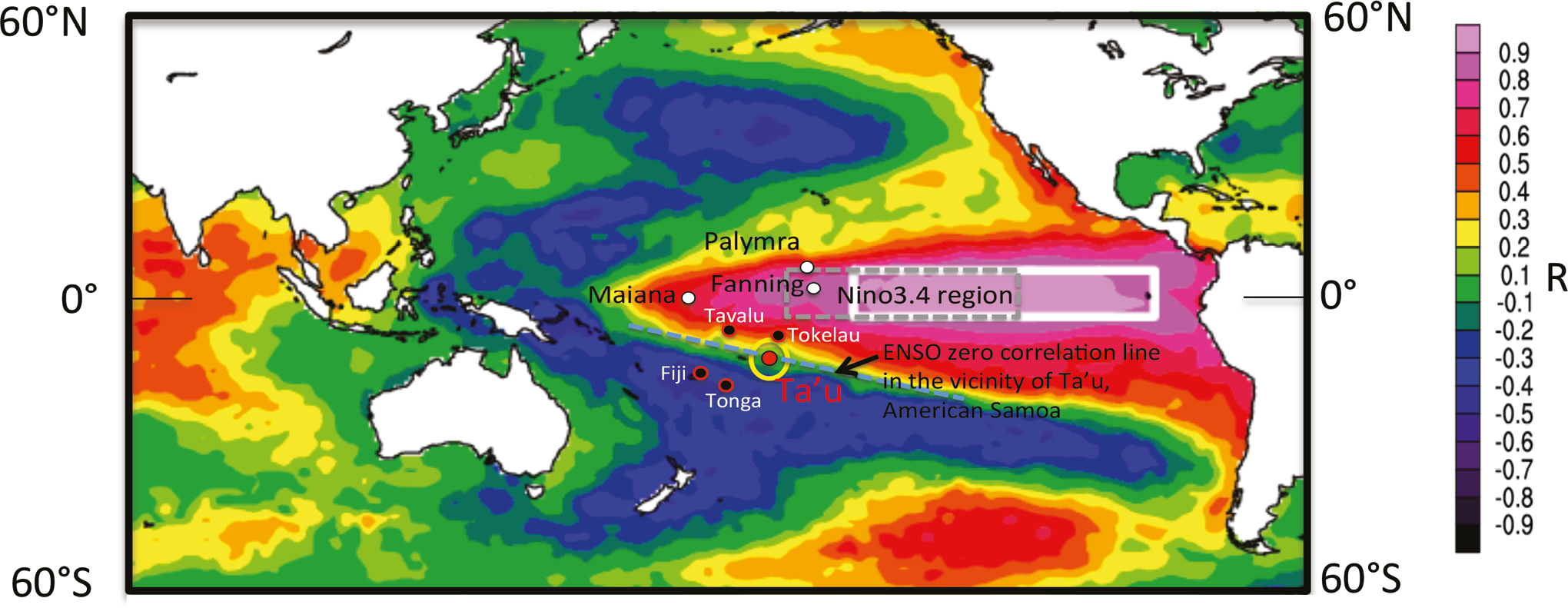
Figure 1: Average correlation pattern of SST to Nino3 SST. Red-purple colors indicate positive correlation and green-blue colors indicate negative correlation. White box indicates the Nino3 region for monitoring ENSO sign and strength and black dashed box the Nino3.4 region. Yellow circle highlights the location of our Ta’u coral site in American Samoa. Note that the zero correlation line (nodal line) runs SE-NW right through Samoa. Also shown are the locations of Fanning, Palmyra and Maiana (see Fig. 3C) and Fiji, Tonga, Tokelau and Tavalu (see Fig. 4). |
During El Niño and La Niña events in the Pacific, the largest SST anomalies are focused in an elongated E-W pattern or footprint that is generally symmetric around 0° latitude in the central Pacific. Individual ENSO events display differences in both the amplitude and the longitude of the largest SST anomalies and cluster analysis of the last 50 years of Pacific SST data indicate that there are three primary El Niño patterns and one primary La Niña pattern (Chen et al., 2015). The mean of these ENSO event patterns results in the classic footprint in ENSO-related SST anomalies surrounded by a perimeter where SST is on average not positively or negatively correlated with ENSO (see Fig. 1). This perimeter reflects a nodal line where on average SST variability is not correlated to ENSO. Instrumental data suggest that the average ENSO nodal line for all types of El Niño and La Niño events has been relatively stable over the last ~50 years.
In the South Pacific, the ENSO nodal line runs northwest to southeast though Samoa (14°S, 172°W) and American Samoa (14°S, 169.5°W) to French Polynesia (17°S, 150°W)(Fig. 1). This location is nearly identical to the nodal line for the decadal mode of SST variability in the Pacific (the Pacific Decadal Oscillation (PDO)). Since the PDO appears to have both subtropical and tropical origins (Newman et al., 2016), the congruence of ENSO and PDO nodal lines in some regions is not unexpected. This region in the South Pacific is also the central rainfall axis of the South Pacific Convergence Zone (SPCZ) which trends northwest to southeast from the Equator in the western Pacific through Samoa and American Samoa.
The SPCZ is the largest spur of the Intertropical Convergence Zone (ITCZ) and a key hydrologic feature in the tropics yet its dynamics and even current position are poorly represented in climate models (Vincent 1994; Vincent et al., 2009; Cai et al., 2012; Evans et al., 2015). Atmospheric data indicate a close relationship between SPCZ movements and ENSO in this region. Over the last 30 years, instrumental precipitation data indicate that during most El Niño events the SPCZ moves a few degrees northward (Gouriou and Delcroix 2002; Vincent et al., 2009; Salinger et al., 1995). Southward SPCZ shifts occur during La Niña events (Gouriou and Delcroix 2002, Vincent et al., 2009; Cai et al., 2012). During very strong El Niño events such as 1982/83 and 1997/98, and during some moderate strength El Niño’s such as 1991-1992, the SPCZ can collapse onto the equator (so-called zonal SPCZ events; Vincent et al., 2009; Linsley et al., 2017). Both SPCZ responses during El Niño result in saltier and slightly cooler conditions on average in the area of the SPCZ central rainfall axis as the SPCZ shifts northeast and the westward flowing South Equatorial Current (SEC) advects relatively salty water into the region.
In an effort to track past changes in the SPCZ response to ENSO events and the PDO we have analyzed sub-seasonal skeletal δ18O in a Porites lutea coral core from the island of Ta’u in the Manua Island group on the eastern side of American Samoa. Ta’u Island is located in the center of the SPCZ and on the nodal line region for both ENSO and the PDO. Variability of surface oceanographic conditions in American Samoa are closely related to SEC dynamics and SPCZ movements. This is the first 50+ year coral δ18O reconstruction from Samoa and American Samoa.
Methods
In November 2011 we cored a large colony of Porites lutea on the western side of the island of Ta’u located at S 14° 15' 33.74": W 169° 30' 01.61" (or S 14 15.566, W 169 30.027) on an exposed outer reef in 7.5m (25 feet) of water (water depth to top of coral). Core sections from the Ta’u-1 core were sawed longitudinally in half and 5mm thick slabs cut at Stanford University and shipped to the Lamont-Doherty Earth Observatory (LDEO) for isotopic analysis. At LDEO, slabs were cleaned in a deionized water bath with a probe sonicator (500W, 20kHz). Slabs were then oven dried at 50°C. Once dried, the slabs were X-rayed in an HP cabinet X-ray system (at 35 Kv). The X-ray positives were used to identify growth band orientation and the maximum growth axis down each slab section as a guide to the subsampling path. Subannual samples were hand-drilled from the slabs at 1 mm intervals by excavating a 3 mm wide by 2 mm deep trough with a variable speed Dremel drill fit with a spherical carbide bit.
Sample powders were analyzed on either an Elementar Isoprime mass spectrometer equipped with a dual-inlet and Multiprep or a Themo-Fisher Delta V+ mass spectrometer with dual-inlet and Kiel IV carbonate reaction device. The instruments are in the same laboratory at LDEO and have been cross-calibrated. They use the same CO2 reference gas and dewatered phosphoric acid is made using the same protocols for each instrument. Here we report the δ18O results of the analysis of this upper 2.6m of core (n=2,565 1mm samples). With the Isoprime we dissolved ~80-120 μg coral powder aliquots in ~100% H3PO4 at ~90°C. With the Delta V-Kiel IV we dissolved ~50-80 μg coral powders in ~100% H3PO4 at ~70°C. NBS-19 standards were analyzed 5 to 6 times per day. To assess external precision and sample homogeneity, 209 replicate samples were analyzed (8.2% replication). The standard deviation of NBS-19 standards analyzed was 0.06‰ for δ18O. The average difference of the replicate δ18O analyses was 0.082‰. All results are reported relative to VPDB (in ‰).
The samples from the core’s live-collected top, serve to anchor the chronology for the δ18O series to November 2011. Below this section, annual δ18O minima and maximum were attributed to seasonal maxima and minima in SST, respectively. Verification of this approach comes from pseudo-coral forward modeling where we used instrumental SST and sea surface salinity (SSS) to generate a modeled coral δ18O series from 2008 to 1981 (Fig. 2). This model assumes all variability in coral δ18O at Ta’u is due to SST and SSS. Ta’u-1 annual average coral δ18O and annual average pseudo-coral δ18O significantly correlate (R=0.77; p < 0.001) with annual average correlations between coral δ18O and SST and SSS of -0.58 and 0.64 respectively. This pseudo-coral comparison verifies our chronology and indicates that Porites coral δ18O at Ta’u is a function of both SST and SSS and where interannual changes in SST and SSS have additive effects on interannual coral δ18O variability. This 2.6m section of core extends from November 2011 to ~ January 1800.
Results and Discussion
 |
|
Figure 2: (top): Sea surface temperature (SST) (NCEP) and sea surface salinity (SSS; Delcroix et al., 2011) for the grids containing Ta’u, American Samoa. (bottom): Ta’u coral δ18O from the Ta’u-1 Porites coral core and “pseudo-coral δ18O” calculated from SST and SSS. The very strong (VS) El Niño events of 1982/93 and 1997/98 are indicated by gray shading. During these events the SPCZ collapsed onto the equator (so-called zonal SPCZ events). Annual average δ18O and pseudo-coral δ18O, R = 0.77 (p<0.001). This correspondence demonstrates that coral δ18O at Samoa is accurately recording surface ocean conditions. |
Although on average there is no correlation between SST variability in American Samoa and Nino3.4 or Nino3 SST over the last ~30 years (see Fig. 1), large El Niño events result in elevated SSS in the Samoa region today (Gouriou and Delcroix 2002; Hasson et al., 2013) (see Fig. 2). There has been a close relationship between SPCZ movements, ENSO and the eastern extent of the western Pacific warm pool with the SPCZ shifting northeast during El Niño events and southwest during La Niña events (Gouriou and Delcroix 2002, Vincent et al., 2009). This SPCZ re-positioning results in more saline conditions on average in the Samoa region during El Niño as the SPCZ shifts northeast and the westward flowing SEC advects relatively salty water into the region.
 |
|
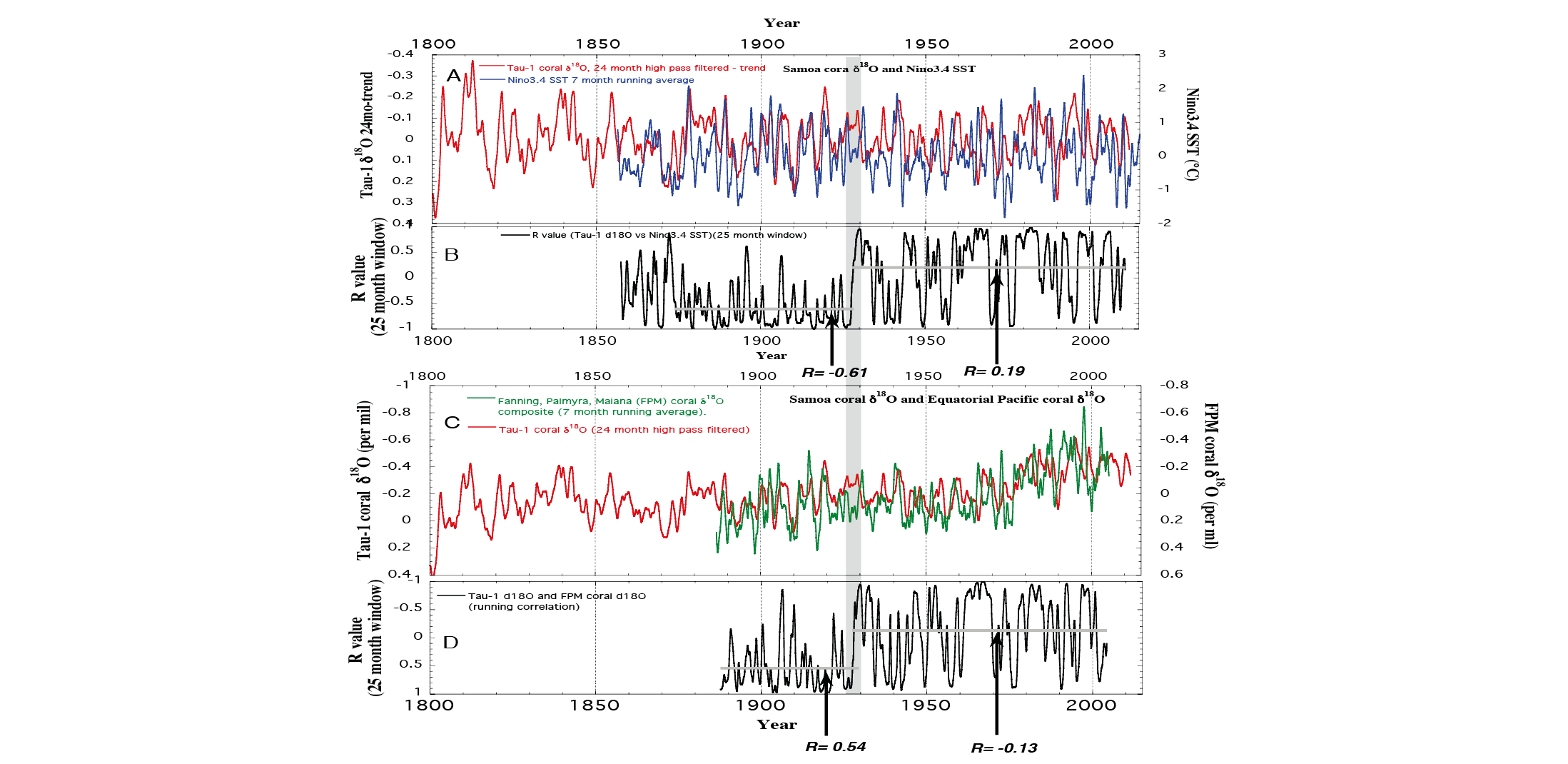
Figure 3: Comparison of Ta’u (American Samoa) coral δ18O to: (A) Nino3.4 SST and (C) an equatorial Pacific composite coral δ18O record from Fanning, Palmyra and Maiana (FPM)(Linsley et al., 2015). Panels B and D show the 25 month running correlation between the series. Horizontal gray bars in B and D indicate average correlation (R value) across the interval. In panel A, arrows indicate El Niño events where it was distinctly cooler and saltier at Samoa. Note that on average after ~1927, warmer conditions in the Niño3.4 area (El Niño) occurred when it was cooler and saltier at Samoa. Before 1927, the opposite pattern is observed; fresher and warmer conditions at Samoa corresponded with El Niño conditions on the equator back to ~ 1872 AD (see panel B) |
To evaluate interannual and lower frequency changes in Ta’u-1 coral δ18O for comparison to equatorial indices of ENSO, we filtered the monthly coral δ18O series in two ways. Our first approach was to 24 month high-pass filter and then detrend the coral δ18O series due to the presence of a significant secular coral δ18O trend. The detrending was accomplished using Singular Spectrum Analysis to isolate and then remove the first principal component (the secular trend). This filtered Ta’u δ18O time series was then compared to 7 month running average filtered Nino3.4 SST anomalies (see Fig. 3A). The second filtering approach was to apply only a 24 month high-pass filter (leaving the trend in place) to facilitate direct comparison to equatorial coral δ18O records (see Fig. 3C). We use a composite average of three coral δ18O records from Fanning (Cobb et al., 2013), Palmyra (Cobb et al., 2013) and Maiana (Urban et al., 2000) as a coral δ18O-based index of equatorial ENSO state (termed FPM; see Linsley et al., 2015).
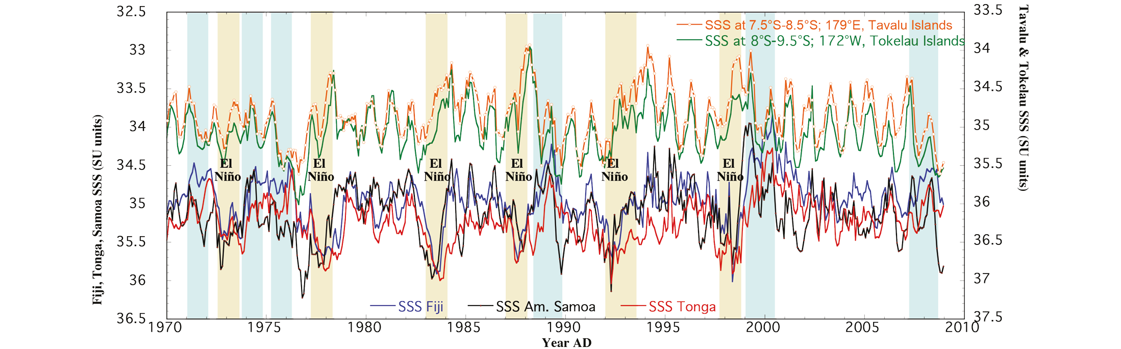
Comparing the Ta’u coral δ18O record to the timing of equatorial ENSO variability indicates a striking phase shift in the decadal mean correlation in the late 1920s. Running correlations between the Ta’u δ18O results and Nino3.4 SST and the FPM equatorial composite coral δ18O highlights the abruptness of the phase shift in the 1920s (see Fig. 3B and D). Sea surface temperature (using ERSST) at American Samoa shows no change in phasing with Nino3.4 SST in the 1920s (not shown) pointing to a change in the timing of interannual surface salinity variability. The Ta’u coral δ18O series indicates that the relationship between El Niño events and more saline conditions in this central region of the SPCZ existed only back to 1927, when there was an abrupt change. Prior to 1927, the Ta’u coral δ18O record contains distinct evidence that on average fresher conditions occurred during El Niño events in Samoa/American Samoa (Fig. 3A and C). This is exactly the situation which occurs today north of Samoa between 7°S and 8°S near the island groups of Tokelau (8°S, 172°W) and Tavalu (7°S, 179°E) (see Fig. 4). Surface salinity is significantly lower during El Niño events in the region extending NW-SE including the Tavalu and Tokelau Island groups at 7-8°S. At the same time, surface salinity increases at Fiji, Tonga and Samoa (Fig. 4).
 |
|
Figure 4: Monthly surface salinity from near Fiji, American Samoa, Tonga, and near Tokelau and Tavalu (north and northwest of Samoa respectively) (data from Delcroix et al., 2011). Note the strong freshening in the regions of the Tokelau and Tavalu Islands during El Niño (tan bars) when the SPCZ shifts northeast. Fiji and Tonga experience higher salinities during El Niño whereas Samoa surface salinity has a more intermediate response. Blue bars are La Niña events. |
These observations indicate that the mean position of the SPCZ must have been shifted southwest of its current position during at least the ~50 year period prior to the late 1920s combined possibly with a reduced latitudinal migration to the northeast during El Niño. This reorganization would explain the fresher conditions during El Niño recorded in our Ta’u coral δ18O record in this period prior to 1927. This is the opposite response to the higher salinity conditions that occur during El Niño events at Ta’u beginning at ~ 1930. The abruptness of the shift in El Niño response in the late 1920s suggests a rapid reorganization of climate patterns in the South Pacific. Based on observational data in the Atlantic, the timing of this abrupt change in SPCZ position occurred during a phase change of the Atlantic Multidecadal Oscillation (AMO) when SST in the North Atlantic abruptly warmed in the mid-1920a as the AMO changed from a negative to positive phase and the ITCZ in the Atlantic shifted north (e.g.; Knight et al., 2006; Zhang and Delworth, 2006; García-García and Ummenhofer 2015).
If the SPCZ central axis also shifted north in the mid-1920s as our Ta’u coral δ18O indicates, this would point to a coordinated ITCZ change in both the Atlantic and Pacific basins. However, the AMO also changed phase in the late 1960s when our Ta’u results do not indicate a phase change between SPCZ variability and equatorial ENSO. The lack of a change in SPCZ-ENSO phasing in the late 1960s when the AMO shifted from a positive phase to a negative phase suggests that there was something climatically different in the late 1920s and/or that the SPCZ and ITCZ are not connected causally. The 1920s were also a time when the PDO changed phase, although this phase change was gradual and appears to have started in the early 1920s. Other clues to significant tropical-subtropical re-organization in the late 1920s at the same time as the SPCZ and Atlantic ITCZ shifted north are a 1920s shift to weaker Pacific trade winds (Thompson et al., 2014). Further interpretation of these preliminary observations of SPCZ position change in the late 1920s will require future work.
affiliations
1 Lamont-Doherty Earth Observatory, 61 Route 9W, Palisades, NY 10964, USA
2 Department of Environmental Earth Systems Science, Stanford University, Stanford, CA, 94305, USA
3 Laboratoire d'Océanographie et du Climat: LOCEAN - IPSL, UMR 7159 CNRS/UPMC/IRD, Université P. et M. Curie, 4 place Jussieu, 75252 Paris cedex 05, France
references
Hugues Goosse1, François Klein1, Didier Swingedouw2, Pablo Ortega3
Introduction
The climatic observations over the instrumental era as commonly defined (from roughly C.E. 1850 to present) cover a period too short to document the full range of climate variability. The study of paleoclimates provides a longer perspective allowing to explore the behavior of the climate system in a wider range of conditions and forcings. The most recent millennium is characterized by a climate very close to the present one and offers a large amount of long paleo-climatic time series. This allows multiple applications, such as to characterize more precisely the decadal to centennial climate variations, to test the robustness of potential mechanisms, or to estimate the exact probability and return period of some specific events. It can also be used to define a baseline climate on which the anthropogenic forcing has imposed its imprint. Fortunately, the last millennium is a period for which we have a relatively large amount of paleo data, with generally a low uncertainty on the dating of the records, and reasonable estimates of the changes in external forcing. Consequently, it has received a lot of attention over the last 20 years, allowing to obtain some crucial results for our understanding of the climate system.
Paleoclimatology requires collaboration between communities as the records are coming from diverse natural archives such as corals, tree rings, ocean and ice cores, speleothems, and others. Deciphering the climate signal in those archives requires a deep understanding of the physical, chemical and biological processes resulting in the formation of those archives. This knowledge is essential for paleoclimate reconstructions but, in turn, gives precious evidence of the impact of climate on natural systems. Furthermore, multi-proxy studies are always desirable so that inherent biases to each of the different archives can be partly canceled out. Studying the last millennium is thus a good opportunity to strengthen the link between the groups focusing on climate changes and the ones working on systems influenced by climate.
In this short note, we briefly present a few illustrations focusing first on the relative contributions of anthropogenic forcing, natural forcing and internal variability in the estimated temperature changes over the last millennium. Specific points about the role of oceanic circulation in the variability at decadal to centennial time scale and the impact of the forcing on climatic modes are then presented. We conclude with some perspectives for future developments.
The warming during the 20th century compared to the pre-industrial climate
A first clear conclusion from the analysis of the last millennium is that at the global scale climate was relatively stable before the industrial era (especially as compared to abrupt climate variations during glacial period), although reconstructions for the last millennium display some significant regional fluctuations. In many regions, the first centuries of the second millennium were relatively warm (the so-called medieval climate anomaly around 950-1250), followed by a colder period (the little ice age, around roughly 1450-1850) (Mann et al., 2009; PAGES 2k consortium, 2013). Those warm conditions during the medieval climate anomaly were less homogenous than during the 20th century, which appears as the only one over the past centuries characterized by a clear warming over all the continents, except Antarctica (Mann et al., 2009; PAGES 2k consortium, 2013). Model results agree with this conclusion and reproduce relatively well the main characteristics of reconstructed changes (Masson-Delmotte et al., 2013; PAGES 2k-PMIP3, 2015). This reinforces our confidence in their ability to reproduce the dominant processes responsible for the continental and global-scale temperature fluctuations at interannual to centennial timescales.
Role of internal variability
An emerging point from the analysis of last millennium climate is the dominant contribution of the internal variability (defined here simply as the one occurring even in the absence of natural or anthropogenic forcing) in the recorded fluctuations. Indeed, internal climate variability often overwhelms completely the influence of the natural external forcing (solar variations, volcanic eruptions) at the local to regional scales in climate model simulations (Goosse et al., 2005; Jungclaus et al., 2010).
Due to this important contribution of internal climate variability, ensembles of simulations, driven by the same external forcing but using different initial conditions, are required for meaningful comparisons between the results of one model and reconstructions and to disentangle the forced and unforced components of the simulated response (Goosse et al., 2005; Jungclaus et al., 2010; Otto-Bliesner et al., 2016).
 |
|
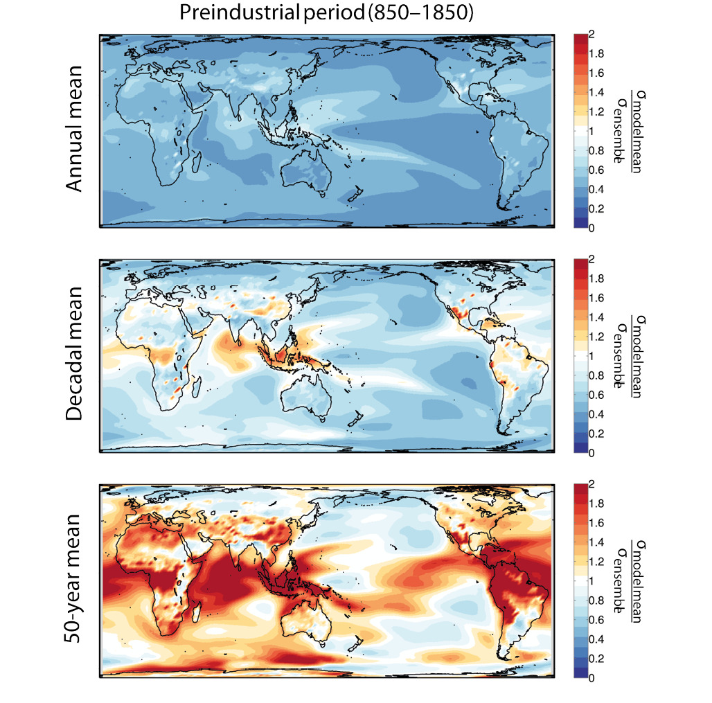
Figure 1: Ratio of the standard deviation of the ensemble mean of an ensemble of 10 simulations performed with CESM1 (Otto-Bliesner et al., 2016) over the mean standard deviation of the ensemble members around this ensemble mean, for the 2-meter air temperature. The standard deviations are computed over the period C.E. 850-1850 for (top panel) annual mean values (middle panel) decadal-means and (bottom panel) 50-year means. The ensemble mean is representative of the forced response while the range of the ensemble around this ensemble mean provides an estimate of the internal variability as simulated by the model. |
A commonly used metric to quantify the relative contribution of forced and internal variability in an ensemble of simulations is the ratio of the standard deviation of the ensemble mean over the mean standard deviation of the individual departures around this ensemble mean. The forced signal dominates in regions where this ratio is larger than 1, and the internally-driven signal when it is lower. These relative contributions can change depending on the timescale considered, as illustrated in Fig. 1 for the 2-meter air temperature in a set of ten last millennium simulations from the climate model CESM1 (Otto-Bliesner et al., 2016). At interannual timescales, internal fluctuations are dominant everywhere while, mainly in the tropics, a larger contribution of the response to the forcings can be found at multidecadal timescales (i.e. 50-year means). The surface average of the ratios over the Northern Hemisphere for annual means, decadal means and 50-year means are 0.45, 0.77 and 1.25, respectively. The corresponding values for the Southern Hemisphere are 0.44, 0.72 and 1.27. For the hemispheric mean temperatures (i.e., when the surface average is computed first before estimating the standard deviations), the relative contribution of the forced response is much larger with ratios of 1.13, 1.72 and 2.53 for the Northern Hemisphere mean temperature and 0.75, 1.58 and 2.66 for the Southern Hemisphere mean.
Many studies have also emphasized the role of internal variability in recent and future changes (Hawkins and Sutton, 2009; Boer, 2011; Deser et al., 2014), even though the external forcing will likely be much larger in the future (compared to the 850-1850 period) due to large anthropogenic greenhouse gases emissions. The last millennium therefore provides an ideal baseline to estimate the magnitude of natural and of internal variability at various spatial and temporal scales. For instance, this period can be used to evaluate the probability of extreme events such as droughts or floods before the dominant impact of greenhouse gas forcing, and the processes responsible for these events, as well as to test the stationarity of the teleconnections within the climate system (e.g., PAGES 2k Consortium, 2013; Ortega et al., 2015; Coats et al., 2016).
The influence of the natural forcing
Although natural forcing may be relatively weak at the regional scale, it is possible to detect and attribute statistically its influence on North Hemisphere temperature during the last millennium, in particular the imprint of volcanic forcing (Schurer et al., 2013). Major volcanic eruptions induce a global-scale cooling in the years following an event. Furthermore, changes in the frequency of the eruptions and their cumulative effects are also responsible for a significant part of the temperature difference between the medieval climate anomaly and the little ice age (Schurer et al., 2013; McGregor et al., 2015).
It has been mentioned above that model results overall agree with reconstructions but a more detailed analysis indicates that many of them tend to simulate a response to volcanic eruptions that is larger than in the reconstructions, with the largest differences in the Southern Hemisphere (Neukom et al., 2014; PAGES 2k-PMIP3, 2015). The correlation of temperature changes among the continents and between the hemispheres is also higher in the model simulations than in the reconstructions (Neukom et al., 2014; PAGES 2k-PMIP3, 2015). This high spatial coherence may be due either to uncertainties in the external forcing estimates, to a too strong and homogenous response to external forcings in the climate model simulations (Stoffel et al., 2015; LeGrande et al., 2016), or to an underestimation of the magnitude of internal variability in the models (which induces changes much less coherent among continents than the external forcings). Alternatively, uncertainty in the proxy-based reconstructions, due to the non-climatic noise, could lead to an underestimation of the coherency of the changes between regions. Determining the origin of those discrepancies will require to investigate all those elements simultaneously. A more objective model-data comparison is in particular required, including forward modules that simulate explicitly the proxy variables measured such as tree ring width or isotope composition (Evans et al., 2013). Indeed, a significant part of the mismatch may simply come from the differences in the variables that are compared between proxies and models.
Changes in ocean circulation
The changes in ocean circulation could potentially provide large contributions to the decadal variability over the last millennium. In the North Atlantic, some model results and reconstructions have suggested that decadal to centennial variations in the intensity of both the subpolar gyres and the meridional overturning circulation induced important changes in the oceanic heat transport, and thus had large-scale impacts on climate (e.g., Lund et al., 2006; McCarthy et al., 2015; Moreno-Chamarro et al., 2016).
Confirming those hypotheses about the role of ocean circulation is a challenge because the available proxy data is much more abundant over the continents than over the ocean and globally only a few marine records have high enough resolution to correctly represent decadal fluctuations. Compilations of observations have confirmed a global oceanic cooling over the period 850-1850, compatible with the one reconstructed for the continents (McGregor et al., 2015). At regional scales, new high-resolution oceanic observations (e.g. Reynolds et al., 2016) and syntheses (as in McGregor et al., 2015) are under way and significant progresses on our understanding of past oceanic changes are expected in the coming years.
The influence of the external forcing on the modes of climatic variability
The climate system variability is organized in large-scale modes of variability that are mainly governed by the dynamics of the ocean and the atmosphere. Well-known examples of these variability modes are the El-Niño Southern Oscillation (ENSO), the North Atlantic Oscillation (NAO) or the Atlantic Multidecadal Variability (AMV). While ENSO impacts the variability of the tropical Pacific, with many teleconnections world-wide, the NAO is focussed on local wind variations in the North Atlantic sector, and the AMV on sea-surface temperature variability in the Atlantic, potentially related with the large-scale Atlantic meridional overturning circulation (AMOC).
 |
|
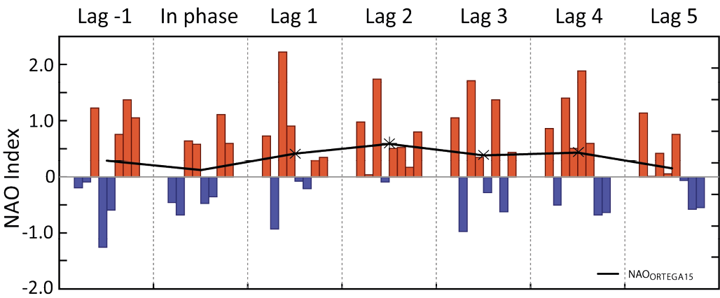
Figure 2: Composite (black line) and individual (colored bars) NAO responses to 8 of the strongest eruptions in the last millennium, as described by a multi-proxy NAO reconstruction covering this period (Ortega et al., 2015). Note that compared to Ortega et al. (2015), we have refined the selection of events to only consider those for which the date of the eruption is well constrained (see Swingedouw et al, 2017). Significance is assessed following a Monte Carlo approach with 1,000 random selections of 8 years from the NAO reconstruction. Significant values at the 90% and 95% confidence levels are represented by crosses and stars, respectively. |
Volcanic eruptions, by cooling the climate at the global scale, might strongly impact the fates of these variability modes and trigger a phase shift. The instrumental era is clearly too short to draw robust conclusions on such potential responses, as it mainly includes five large volcanic eruptions (Krakatau in 1883, Santa María in 1902, Agung in 1963, El Chichón in 1982 and Pinatubo in 1991). On the basis of analyses over the last millennium, some indications exist that volcanic eruptions might promote a positive phase of ENSO the year following a large eruption (e.g., Emile-Geay et al., 2008). Similarly, it has been recently shown that the largest eruptions of the last millennium are almost systematically followed by a positive phase of the NAO, particularly clear for the second winter after the eruptions (Ortega et al., 2015, Fig. 2). For the AMV and AMOC, a few recent studies suggest that volcanic eruptions may act as a pacemaker of their decadal variability over the last millennium (Otterå et al., 2011; Swingedouw et al., 2015). Nevertheless, no entirely clear and robust conclusions concerning the exact impact of volcanic eruptions on these variability modes can be drawn, notably due to difficulties of climate models to reproduce such impacts and the intricacy to separate the contribution of the forcing from the stochastic internal fluctuations (Swingedouw et al., 2017).
Further developments and perspectives
A promising way forward to reduce the uncertainties is the combination of paleo-data and model results to reconstruct as accurately as possible the state of the system over the past millennium. Although many challenges remain, such reanalyses for the past millennium are currently under development (Goosse et al., 2012; Hakim et al., 2016; PAGES, 2017). In addition to contributing to a better understanding of the dynamics of the system, those reconstructions could provide a test bed, complementary to the last century, for decadal prediction systems (Meehl et al., 2014), in order to evaluate their skill in a wider range of conditions. However, the ability to generate the initial climatic conditions for such retrospective predictions (hindcasts) is a dominant issue and the small amount of available data, notably in the ocean realm, strongly limits for the moment the breadth of the tests that can be performed over these past periods.
Many of the conclusions and the questions raised above for the last millennium correspond to research priorities for the more recent past (i.e., the instrumental period) as well. The advantage of the investigations covering the last millennium is the possibility to analyze longer time series, and thus increase the signal-to-noise ratio for the detection and attribution, for example, of forced signals. The disadvantage compared to the instrumental period is the scarcity and larger uncertainties of the proxy records and the larger resources needed to perform model simulations spanning several centuries. Despite those challenges, the information brought by the instrumental and pre-instrumental periods is very complementary, justifying strong interactions and collaborations.
acknowledgements
Hugues Goosse is Research Director within the Fonds National de la Recherche Scientifique (F.R.S.-FNRS-Belgium). Didier Swingedouw is supported by the French Centre National de la Recherche Scientifique (CNRS). The work of Pablo Ortega is funded by the NERC research Project DYNAMOC (NE/ M005127/1). This note is a contribution to the PAGES2k working group of PAGES. Support for PAGES activities is provided by the US and Swiss National Science Foundations, US National Oceanographic and Atmospheric Administration and by the Future Earth program.
affiliations
1 ELIC/TECLIM Université catholique de Louvain, Belgium
2 Environnements et Paléoenvironnements Océaniques et Continentaux (EPOC), UMR CNRS 5805 EPOC—OASU—Université de Bordeaux, Allée Geoffroy Saint-Hilaire, Pessac 33615, France
3 NCAS-Climate, Meteorology Department, University of Reading, UK
references
Haiyan Teng, Gerald A. Meehl, Grant Branstator, Stephen Yeager, Alicia Karspeck
Introduction
Initialized predictions tend to drift away from the initial states towards the model’s imperfect climatology. If all predictions drift in a coherent manner that is independent of an initial state, the drift to a large extent can be removed during the posterior bias correction. However, lack of continuous global ocean observations poses a serious challenge to the quality of ocean initial states that span several decades. Furthermore, incoherent initial errors especially in the Tropics can be amplified by air-sea coupling as a prediction evolves and can impact the entire globe through atmospheric teleconnections. Consequently the effect of such initial shocks on predictions are difficult to remove by simple bias correction methods and can overwhelm the relatively small decadal signals that we seek to predict. Here, we describe the initialization shock in a set of decadal prediction experiments with the Community Climate System Model version 4 (CCSM4) and discuss the challenges they cause to near-term hindcasts, in particular of the Interdecadal Pacific Oscillation (IPO).
CCSM4 decadal prediction experiments
CCSM4 is a fully coupled general circulation model consisting of atmosphere, ocean, land, and sea ice that are linked via a flux coupler and no flux corrections are employed (Gent et al., 2011). The atmosphere model uses a finite volume dynamical core with a nominal horizontal resolution of 1°and 26 layers in the vertical. The ocean is a version of the Parallel Ocean Program (POP) with a nominal latitude-longitude resolution of 1° (tapering down to 1/4° in latitude in the equatorial tropics) and 60 levels in the vertical. The land and sea ice components share the same horizontal grids as the atmosphere and ocean models, respectively.
The CCSM4 decadal prediction experiments (also referred to as initialized hindcasts, or hindcasts) analyzed here are an expansion of a previously documented set (Yeager et al., 2012) that was submitted to the Coupled Model Intercomparison Project phase 5 (CMIP5) (Taylor et al., 2012). The ocean/sea ice initial conditions are obtained from a CCSM4 ocean/sea ice stand-alone simulation forced with atmospheric variables, such as surface winds, air temperature, precipitation, surface fluxes, sea level pressure, humidity etc. from the NCEP/NCAR reanalysis (Kalnay et al., 1996). This forced ocean/ice simulation represents the NCAR contribution to the Coordinated Ocean-ice Reference Experiments phase II (CORE II) (Danabasoglu et al., 2014). The initial states for atmosphere/land are taken from CCSM4 CMIP5 uninitialized historical/RCP4.5 runs. For each January 1st during 1955-2014, we ran a 10-member ensemble of initialized hindcast experiments with the ensemble spread created by perturbing the atmosphere (or both atmosphere and land in the earlier set as documented by Yeager et al., 2012) initial conditions.
There exists a large variety of bias correction methods and they are designed to reduce errors and add skills to the forecasts. To avoid complexities that can arise in assessing the source of improvements in calibrated initialized hindcasts compared to the traditional climate change projection experiments without initialization (also referred to as the uninitialized simulations), here we examine interannual anomalies with respect to a hindcast climatology that is only a function of prediction range; no observations are taken into account in our calculation of anomalies (as in Doblas-Reyes et al., 2013). That is, at lead t (t=Month1, 2, …, 120) from a start year j (j=year 1955, ..., 2014), the interannual anomalies

where ![]() is the raw hindcast, and N is the total number of start years. By using this methodology, the reference model hindcast climatology
is the raw hindcast, and N is the total number of start years. By using this methodology, the reference model hindcast climatology ![]() already includes most model systematic errors (including systemic errors in the forced response, assuming the forced response is independent to the initial states). Presuming initial errors are the same for different start years, computing differences on the right hand side of (1) will leave mostly the signal in the hindcasts. A caveat is that the initial errors often vary with start years, which is even more true for decadal predictions than for seasonal predictions, as the former covers decades with limited ocean observations.
already includes most model systematic errors (including systemic errors in the forced response, assuming the forced response is independent to the initial states). Presuming initial errors are the same for different start years, computing differences on the right hand side of (1) will leave mostly the signal in the hindcasts. A caveat is that the initial errors often vary with start years, which is even more true for decadal predictions than for seasonal predictions, as the former covers decades with limited ocean observations.
Warm shocks in the Nino3.4 SST
First, we focus on sea surface temperature (SST) in the Nino3.4 region for the hindcast behavior. Fig. 1a shows the time evolution of raw Nino3.4 SST during the 10-year hindcast period; with each colored thin line representing a raw 10-member ensemble mean hindcast from a start year indicated by the label bar, and the thick black line representing the observed climatology (http://www.esrl.noaa.gov/psd/gcos_wgsp/Timeseries/Data/nino34.long.data). Strikingly, the Nino3.4 SSTs from hindcasts initialized during the early decades (1955-1970, dark blue) tend to produce a 2°C warm spike relative to the observed climatology in the first two or three years. By contrast there are no obvious warm spikes in the later start years, and a number of hindcasts initialized around year 2000 produce cold spikes of roughly -2°C in the first three years.
 |
|
Figure 1: (a) Time evolution of raw Nino3.4 SST during the 10-year hindcast period, with each colored thin line representing a 10-member ensemble mean hindcast from a start year indicated by the label bar, and the thick black line representing the observed climatology. The hindcast SSTs are smoothed by an unweighted 6-month running average. b-d) interannual Nino3.4 SST anomalies from the CCSM4 hindcasts (red) and observations (black) at three different forecast ranges: (b) Month 1, (c) Year 2 and (d) Year 3-7. |
We further examine the hindcasts of Nino3.4 SST at three different lead times by comparing predicted interannual anomalies defined by (1) to observed anomalies derived by subtracting the observed climatological mean. In Month1 (Fig.1b), the hindcast anomalies (red) generally match the observations (black). This reflects the consistency of the initial states with the observations. Because we cannot effectively remove the initial shock that is most pronounced in Year 2 with the calculation in (1), the Year 2 annual mean Nino3.4 SST hindcast anomalies show a pronounced multidecadal shift, with more than 1°C anomalies in the early two decades and -1°C anomalies in late 1990s and the early 2000s (Fig. 1c). The observed anomalies do not have these multidecadal variations suggesting that the variations are examples of impacts from initialization shocks that cannot be removed by simple bias correction techniques.
Year 3-7 is the forecast range that some current decadal prediction experiments aim to target (Meehl et al., 2014a, 2014b, 2016; Meehl and Teng, 2012, 2014a, 2014b). The tropical Pacific, which is a pace-maker of global climate (Kosaka and Xie, 2013), has limited initial-value predictability for all initial states at this range of 3-7 years based on a “perfect model” assessment (Branstator and Teng, 2010). When we calculate the Nino3.4 SST interannual anomalies at the Year 3-7 range (Fig.1d), we still find secular multidecadal variability, with a downward trend until about 1980, and then stable or somewhat upward after that. In some ways this is reminiscent of the Year 2 drifts (Fig. 1c). Note there is a change in the range of the y-axis from Fig.1bc to Fig.1d; the amplitude of the Year 3-7 anomalies is much weaker.
What caused the shock?
 |
|
Figure 2: Start year vs. longitude distribution of Month1 (top) and Year1 (bottom) errors in equatorial SST (5°S-5°N) and 20°C isotherm depth (Z20, 2°S-2°N). Boundaries for the Nino3.4 region are outlined by the two vertical dashed lines. The observed SST and Z20 are obtained from HadISST (Rayner et al. 2003) and 2009 World Ocean Database. |
First, we examine how closely the ocean initial conditions reflect observations by comparing the Month1 hindcasts and the corresponding January observations. We focus on SST and subsurface temperature measured by the thermocline depth (20°C isotherm, Z20) in the equatorial Pacific, with the observed SST obtained from HadISST (Rayner et al., 2003) and the Z20 observations calculated from the 2009 World Ocean Database (Levitus et al., 2009). Our main focus is not climatological meanbiases but a possible change in either the strength or distribution of the initial errors occurring at about 1980 that might explain why the positive initial shock only occurs for start years between roughly 1955-1970.
The warm spikes in the Nino3.4 region in the early hindcast period do not seem to be directly caused in any obvious way by the SST initial errors, for those initial errors are generally negative (~ -1°C) during 1950-1970 and are actually cooler than the errors in start years after 1980 (Fig. 2a). However, the Z20 errors are much deeper in the pre-1980 initial conditions compared with the later period (Fig. 2b), indicating that the early start years have a much warmer subsurface temperature bias (hence deeper Z20). This subsurface warm bias is further amplified during Year 1 (Fig. 2d) and appears to have propagated to the surface (Fig. 2c).
We further diagnose the interannual temperature tendency budget in the upper 100m in the Nino3.4 region:

where T is the depth averaged temperature anomaly, Qnet is the net air-sea surface flux. H, ρ0, and Cp are three constants that denote the layer thickness (=100m, and consistent results are found for H=60m), water density, and heat capacity, respectively. UETW-E and VNTS-N denote horizontal and meridional convergence (differential at the west and east boundary, or the south and north boundary of the Nino3.4 region) of temperature flux respectively, and WTT100m is the vertical temperature flux at the 100m depth. Prime represents the interannual anomalies (1). The residual term includes tendencies from the diffusive temperature fluxes and fluxes from the subgrid scale.
 |
|
Figure 3: Budget analysis for the mixed layer temperature tendency anomalies in the Nino3.4 region averaged in a) Month1-3 and b) Month 6-12 hindcasts. All terms are shown as interannual anomalies, including temperature tendency (red), surface flux (orange), horizontal (UET, blue) and meridional (VNT, green) convergence of temperature flux, temperature flux at the 100m depth (WTT, purple), and sum of SHF, UET, VNT and WTT (black dashed). All curves are smoothed by the 10-year running averages. |
During the first three months, the positive interannual temperature tendency (Fig. 3a, red), which is contributing to the warm spikes seen in Fig.1a, can be well explained by the first four terms on the right hand side of the tendency equation. (In Fig. 3a, the sum of the four terms is represented by the black dashed line). Both the vertical temperature flux at the bottom of the layer (purple, Fig. 3a) and the meridional temperature flux convergence (green, Fig. 3a) make positive contributions to the positive temperature tendency anomalies during the 1955-1975 start years, which are partially compensated by a large negative zonal temperature flux convergence (blue, Fig. 3a).
More specifically, interannual anomalies in both vertical velocity and temperature at the 100m depth contribute to the anomalously large WTT'100m during 1955-1975 in each of the first three months (not shown). Although we don’t have reliable ocean observations to quantify the observed decadal change in the equatorial upwelling velocities, the domain averaged vertical velocity at 100m depth in the Nino3.4 region in Month 1 of the hindcasts is significantly higher (at the 99% confidence level) during the first two decades (1955-1974) compared to the last two decades (1995-2014), with the 20-year mean equal to 0.51 m/day and 0.38 m/day, respectively. Meanwhile, the corresponding 100m depth temperature during the two periods is 25.0°C and 24.2°C, respectively; the former period is significantly warmer at the 98% confidence level than the later period.
Once the warm subsurface temperature anomalies are advected into the mixed layer and the surface warming is fully established for all start years during 1955-1975 by Month 6 (not shown), the mixed layer warming is further amplified through atmosphere-ocean coupling. This is indicated by the Month 6-12 anomalous temperature tendency during 1955-1975 being mainly produced by the UET'w-E term, which is partially compensated by the other four terms on the right hand side of the temperature tendency equation (Fig. 3b). Positive UET'w-E is expected from westerly wind anomalies induced by the warm SST anomalies, and in a figure not shown we find the climatological zonal temperature gradient advected by the anomalous zonal current can explain a large portion of the positive temperature tendency anomalies during 1955-1975 (red, Fig. 3b). Associated with westerly surface wind anomalies are equatorial downwelling anomalies and meridional temperature divergence which make WTT'100m and VNT'S-N negative.
While the budget analysis can explain how the warm spikes in the pre-1975 hindcasts are triggered and amplified, it does not single out which atmospheric forcing from the NCEP/NCAR reanalysis has played a key role in producing these ocean initial conditions. Among more than a dozen models that participated in the CMIP5 decadal prediction experiments (Kirtman et al., 2013), the Max Planck Institute Earth System Model (MPI-ESM) has a similar initial shock problem to that found in CCSM4. Their ocean initial conditions were also produced by forcing the ocean-only model with the NCEP/NCAR reanalysis. Pohlmann et al. (2016) further pin down the origins of the shock in this model to a spurious change in the NCEP/NCAR surface wind stress over 150°W-120°W, 10°S-10°N, which is strongly westward before the 1970s and eastward after 1980 compared to other reanalyses. The anomalous trade wind trend in the NCEP/NCAR reanalysis may help to explain the CCSM4 initialization shock because: a) through Ekman transport, the anomalously strong equatorial trade wind stress before the 1970s in the NCEP/NCAR reanalysis can directly induce anomalous equatorial upwelling in the CCSM4 initial states; b) in an investigation at NCAR parallel to that done at MPI, a new set of decadal prediction experiments were produced from an ocean state reconstruction generated using a different wind field (20th Century Reanalysis, Compo et al. 2006) than the prior CORE-II simulation. We find no spurious pre-1975 subsurface warming in the new ocean initial conditions. Therefore, it is likely that those especially warm subsurface initial conditions pre-1975 in CCSM4 are also caused by the NCEP/NCAR spurious wind stress. More importantly, our preliminary analysis of new hindcast experiments initialized from the ocean states produced by the 20th Century Reanalysis winds indicates no big initialization shock.
Impacts on the IPO hindcast
One might hope the model can adjust quickly to the initialization shock in the equatorial Pacific so that for the near-term forecast range (e.g. 3-5 years) it is still possible to harvest some skill from modes or patterns that have long predictability. Indeed, the CCSM4 experiments show considerable skill in predicting North Atlantic upper-ocean heat content and surface temperature up to a decade in advance (Yeager et al., 2012; Karspeck et al., 2015), which is consistent with other models’ CMIP5 near-term climate predictions (Doblas-Reyes et al., 2013; Kirtman et al., 2013). There also is skill in hindcast simulations of the IPO SST pattern in terms of model anomalies computed from observations (Meehl et al., 2014; Meehl et al., 2016). However, also consistent with other models, Fig. 1d indicates prediction skill is low in the year 3-5 equatorial Pacific SST in CCSM4, raising the issue of how hindcast skill is evaluated for the Interdecadal Pacific Oscillation (IPO) (Power et al., 1999) on the near-term time scales.
The observed IPO pattern is often defined as the second empirical orthogonal function (EOF) of low-pass filtered Pacific SSTs at 40°S-60°N, 120°E-70°W (Fig. 4a). While the spatial pattern closely resembles the El Nino composite (Zhang et al., 1997), the IPO time series has much lower frequency. It shows a negative-to-positive transition in the mid 1970s, and a positive-to-negative transition in the late 1990s and early 2000s (black line in Figs. 4de). The latter has been regarded as the main cause for the recent slow-down in observed global warming (Easterling and Wehner, 2009, Meehl et al., 2011, 2013). Motivated by the IPO’s strong impact on global climate, and by the fact that it contains a midlatitude component (the Pacific Decadal Oscillation, PDO) (Mantua et al., 1997) that is more predictable than the tropical SSTs (Teng and Branstator, 2011; Branstator and Teng, 2010, 2012; Branstator et al., 2011), predicting the IPO has become a goal for the decadal prediction efforts.
 |
|
Figure 4: (a) The observed IPO: SST anomalies regressed upon the IPO index (second EOF of 10-year low-pass filtered HadISST during 1870-2016, time series shown as the black line in (d) and (e).(b) and (c) regressed EOF1 SST anomalies from CCSM4 Year 2 (b) and Year3-7 (c) hindcasts and the corresponding time series are represented by red thick line (ensemble mean) and orange shading (spread) in d) and e). |
The initialization shock has an impact on Year 2 hindcasts of the IPO in CCSM4. This is shown by an EOF analysis of the Year 2 annual mean SST anomalies over the Pacific Ocean from all start years and all ensemble members. The time series of EOF1 (ensemble average and spread is shown by the red thick line and orange shading in Fig. 4d respectively, and it accounts for 54% of the total variance) shows a downward trend, crossing from positive to negative near year 1980. While both the timing of the cross-over from positive to negative (Fig. 4d) and the amplitude of the regressed SST anomalies (Fig. 4b) in the Nino3.4 region resemble the time series of the Year 2 Nino3.4 interannual anomalies shown in Fig. 1c, the regressed SST anomalies (Fig. 4b) trend, crossing from positive to negative near year 1980. While both the timing of the cross-over from positive to negative (Fig. 4d) and the amplitude of the regressed SST anomalies (Fig. 4b) in the Nino3.4 region resemble the time series of the Year 2 Nino3.4 interannual anomalies shown in Fig. 1c, the regressed SST anomalies (Fig. 4b) further demonstrate that the equatorial SST shock is associated mainly with a trend in the PC time series with a basin-wide IPO-like (or ENSO-like) pattern. Since we don’t find such large cold temperature anomalies in the mixed layer temperature along the Kuroshio extension region in the Month1 hindcasts from 1955-1970, these cold anomalies are likely induced by the initialization shock in the equatorial Pacific through atmospheric teleconnections.
We repeat the EOF analysis for the Year 3-7 annual mean SST anomalies (Figs. 4c and e) and the PC1 also represents a downward trend and a somewhat different timing of the positive to negative change compared to Year 2, with the change occurring somewhat later around 1990-95 (Fig. 4e). This could be due to multi-year smoothing and the longer hindcast range (since the x-axis represents the central prediction year of the five year average range rather than initialization year, e.g. a hindcast for 1986-1990 is represented on the plot as 1988 and was initialized in 1984). At this longer range, the SST anomalies associated with EOF1, representing the trend in the initialized hindcasts, have damped greatly in the equatorial Pacific, but almost no damping is found in the SST anomalies in the North Pacific, possibly due to long persistence resulting from a deeper mixed layer. Thus, despite the fast adjustment in the tropical Pacific, the initialization shock represented by a trend that in some ways resembles an IPO/PDO pattern may persist in the higher latitude oceans. Thus, while the high persistence of midlatitude anomalies has the potential to give longer predictability to anomalies present in the midlatitude initial conditions, it may also degrade predictive skill as it enhances the persistence of anomalies produced by initialization shock.
Our results and those in other investigations (Sanchez-Gomez et al., 2016; Pohlmann et al., 2016) indicate that initialization shock can degrade forecasts and sometimes even produce negative skill. For example, when trying to predict the negative IPO prior to the mid-1970s, the initialization shock shown as a trend in EOF1 of both the Year 2 and Year 3-7 interannual anomalies (Figs. 4d,e) suggests the initial shock would contribute to positive values of the IPO for that time period. Therefore, skill in the positive IPO SST pattern in the CCSM4 hindcasts for this time period relative to observations (Meehl et al., 2014; 2016) could conceivably have been higher if positive values of the initialization shock trend were taken into account. There are also occasions such as in the 1990s when the trends in the Year 3-7 anomalies, which to a large extent may be caused by the initialization shock, are in phase with the observed IPO such that those negative trend values could artificially contribute some skill in hindcasts for the negative phase of the IPO. A better understating of the time-dependent characterization of initialization shock in CCSM4 is thus necessary in order to correctly interpret the model skill.
acknowledgement
We thank Dr. Holger Pohlmann for valuable comments. Portions of this study were supported by the regional and Global Climate Modeling Program (RGCM) of the U. S. Department of Energy’s, Office of Science (BER), Cooperative Agreement DE-FC02-97ER62402, and the National Science Foundation. SY acknowledges support from the National Oceanic and Atmospheric Administration (NOAA) Climate Program Office under Climate Variability and Predictability Program grants NA09OAR4310163 and NA13OAR4310138, and both SY and AK are partly funded by the National Science Foundation (NSF) Collaborative Research EaSM2 grant OCE-1243015. Computing resources were provided by National Center for Atmospheric Research (NCAR)'s Computational and Information Systems Laboratory (CISL), and by the National Energy Research Scientific Computing Center (NERSC) under Contract No. DE-AC02-05CH11231and Oak Ridge Leadership Computing Facility located in the National Center for Computational Sciences (NCCS) at Oak Ridge National Laboratory under Contract DE-AC05-00OR22725, which are supported by BER of the U.S. Department of Energy. NCAR is sponsored by the National Science Foundation.
affiliation
National Center for Atmospheric Research, Boulder, USA
references
Scott Power1, Ramiro Saurral2, Christine Chung1, Rob Colman1, Viatcheslav Kharin3, George Boer3, Joelle Gergis4, Benjamin Henley4, Shayne McGregor5, Julie Arblaster5, Neil Holbrook6, Giovanni Liguori7
Introduction
Multi-year (2-7 years) and decadal climate variability (MDCV) can have a profound influence on lives, livelihoods and economies. Consequently, learning more about the causes of this variability, the extent to which it can be predicted, and the greater the clarity that we can provide on the climatic conditions that will unfold over coming years and decades is a high priority for the research community. This importance is reflected in new initiatives by WCRP, CLIVAR, and in the Decadal Climate Prediction Project (Boer et al., 2016) that target this area of research. Here we briefly examine some of the things we know, and have recently learnt, about the causes and predictability of Southern Hemisphere MDCV (SH MDCV), and current skill in its prediction.
Causes of SH MDCV
As with other parts of the globe, internally generated climate variability is a major element of SH MDCV (Kirtman et al., 2013). Major components of internal variability for the Southern Hemisphere are decadal variations in ENSO, the Interdecadal Pacific Oscillation (IPO, Garreaud and Battisti, 1999; Power et al., 1999; Salinger et al., 2001; Folland et al., 2002; Wu and Hsieh, 2003; Holbrook et al., 2011; Christensen et al., 2013; Kosaka and Xie, 2013; England et al., 2014; Holbrook et al., 2014; Watanabe et al., 2014; Henley et al., 2015; Meehl et al., 2016), the Southern Annular Mode (SAM (Shiotani, 1990; Thompson et al., 2000; Watterson, 2009; Pohl et al., 2009; Yuan and Yonekura, 2011; Jones et al., 2016), and the Indian Ocean Dipole.
North Pacific decadal variability has recently been described by Di Lorenzo et al. (2015) as a seasonally-based red noise process involving the interaction between extratropical atmospheric variability and ENSO via the North Pacific Meridional Modes (Chiang and Vimont, 2004). Although a similar mechanism has not yet been proposed for the South Pacific DCV, tropical-extratropical interactions, including via both the ocean and atmosphere, are thought to be at least partly responsible for inducing decadal to multidecadal variability in the South Pacific too (e.g., McGregor et al., 2007, 2008, 2009a and b; Farneti et al., 2014; Zhang et al., 2014; Ding et al., 2015). Inter-basin interactions are also thought to play a role in driving Pacific Ocean decadal and multi-decadal variability (e.g., McGregor et al., 2014; Kucharski et al., 2016, Chikamoto et al., 2016). Palaeoclimate reconstructions of MDCV in the Pacific vary significantly in their spectral characteristics, likely due to spectral biases in the different proxy records, non-stationarity of teleconnections and the use of various statistical reconstructions methods (Bateup et al., 2015).
External forcing, both natural and anthropogenic, can also drive decadal and longer-term variability in the SH (e.g., Bindoff et al., 2013 and references therein). Natural drivers include volcanic eruptions (e.g. Church et al., 2005), while anthropogenic external drivers include changes in greenhouse gas concentrations, aerosols (Cai et al., 2010) and stratospheric ozone (Kirtman et al., 2013; Arblaster et al., 2014; Eyring et al., 2013).
How well do climate models simulate MDCV in the SH?
The ability of climate models to simulate Earth's climate was assessed in the IPCC Fifth Assessment Report (Flato et al., 2013). They concluded that models reproduce many important modes of variability. This includes modes of relevance to the SH: ENSO, the Indian-Ocean Dipole and the Quasi-Biennial Oscillation. Models have improved in some respects since the last generation although, in the case of ENSO, some of this improvement might not be entirely for the right reasons.
While models are extremely valuable tools that enable us to improve our understanding of SH MDCV, they are not without their limitations. For example, while CMIP5 models tend to capture the spatial pattern of the IPO, models tend to underestimate the magnitude of SST variability associated with the IPO (Power et al., 2016; Henley et al., 2017), and both the magnitude of DCV in trade winds (England et al., 2014; McGregor et al., 2014) and multidecadal changes in the strength of the Walker Circulation (Kociuba and Power, 2015). These deficiencies appear to be due, at least in part, to modeled ENSOs that tend to be too oscillatory on too short a time-scale. This makes it hard for the models to maintain multi-year and longer-term anomalies (Kociuba and Power, 2015; Power et al., 2016).
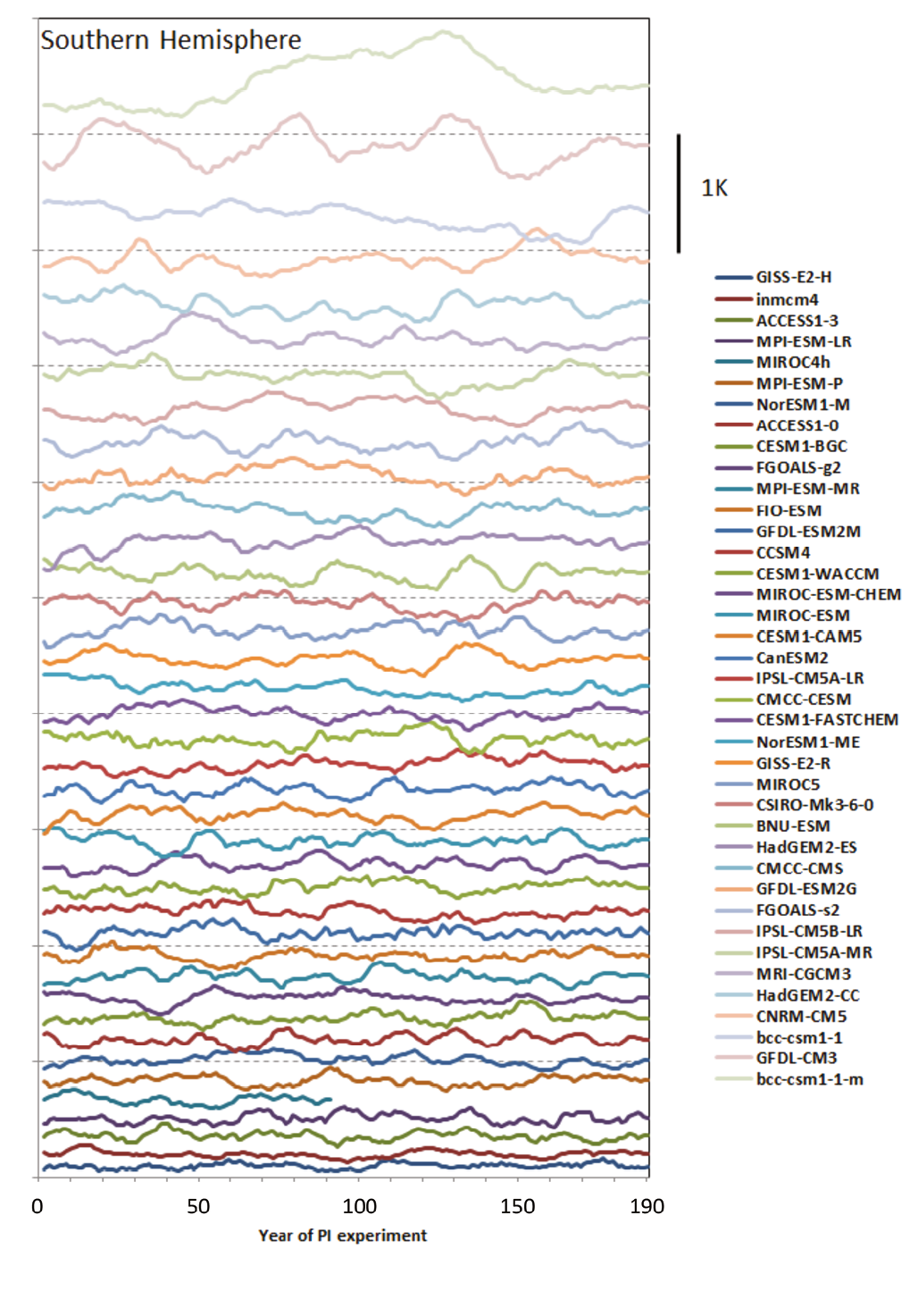 |
|
Figure 1: Time series of the (detrended) 10-year running annual mean surface air temperature, averaged over the SH from the CMIP5 models (K), ordered from smallest to largest. Values calculated from the first 200 years of pre-industrial experiments offsets for display purposes. |
A further illustration of the limitations of CMIP5 models in simulating SH MDCV is seen in Fig. 1. It shows time-series of the decadal variability in SH surface air temperature from pre-industrial runs of CMIP5 models. The model-to-model range in the magnitude and character of the variability is remarkable. Some models exhibit variability that has a range of a few tenths of a degree, while the range of some other models is three or more times larger. The character of the variability also differs markedly among models. In some models there is pronounced multi-decadal variability, whereas in other models variability occurs on much shorter time-scales. While further research is needed to ascertain which of these simulations more realistically captures SH MDCV. Clearly, given the large model to model differences evident in Fig.1, care is needed in assigning confidence to conclusions drawn on the basis of SH MDCV simulated in the current generation of climate models.
There have been other studies investigating SH MDCV of the past 1000 years in climate model simulations and reconstructions For example, a recent study by Hope et al. (2016) examined the decadal characteristics of ENSO spectra based on seven published ENSO reconstructions, and indices of Nino 3.4 SSTs and the Southern Oscillation Index calculated from six CMIP5–PMIP3 last millennium simulations. The post-1850 spectrum of each modelled or reconstructed ENSO series captures the observed spectrum to varying degrees. However, no single model or ENSO reconstruction completely reproduces the instrumental spectral characteristics across the multiyear or decadal bands.
Appreciable changes in the level of decadal ENSO variability is observed in the reconstructions and simulations of the pre-1850 period. While much of this represents internally generated variability (see e.g. Power et al., 2006), some of the variability may be linked to intermittent major volcanic eruptions (Hope et al., 2016). Nevertheless, Hope et al. (2016) report inconsistencies between reconstructions, models and instrumental indices used to evaluate changes over past centuries, reflecting the complexity of reconstructing and simulating past changes of a highly variable coupled system. In the reconstructions, variability arises from internal climate processes, different forced responses, or non-climatic proxy processes that are still not well understood (Ault et al., 2013).
Improving the simulation of SH MDCV would be greatly assisted by the availability of additional data from high latitude regions. The palaeoclimate reconstruction of the SAM by Abram et al. (2014) displays good agreement with CMIP5–PMIP3 last millennium simulations. Although the reconstruction shows a progressive shift towards SAM's positive phase as early as the fifteenth century, the positive trend in the SAM since 1940 is reproduced by multi-model climate simulations forced with rising greenhouse gas levels and ozone depletion (Abram et al.. 2014). These results are likely to reflect the brevity of the instrumental data from high latitudes, and associated deficiencies in model representation of SH climate (Jones et al., 2016).
Predictability of MDCV in the SH
 |
|
Figure 2: The relative importance of initial conditions and external forcing for the climate prediction and predictability of time-averaged temperature in the SH. The correlation skill scores for the ensemble mean of initialized temperature forecasts, and the model-based "potential" correlation skill scores, area averaged over the SH, are presented as orange lines. The same quantities, but for uninitialized climate simulations, are plotted as green lines. All lines represent area-averaged SH values. Solid lines: hindcast skill; Dashed lines: potential skill. Results are for temperature averaged over periods from a month to a decade. (Figure prepared by V.V. Kharin based on the results reported in Boer et al. (2013)). |
In climate science the term “predictability” has a different meaning to “predictive skill”. Predictability provides an estimate of the upper limit to predictive skill, in the absence of technical problems - apart from uncertainty in initial conditions. Predicability is usually estimated from a model’s ability to predict its own evolution given imperfect initial conditions. The presumption is that the results from a well-behaved climate model can provide information on the predictability of the actual climate system. Predictability arises from internal variability, external forcing (e.g. increasing greenhouse gas concentrations), and interactions between them. One estimate of the relative importance of initial conditions and external forcing for the predictability of time-averaged temperature in the Southern Hemisphere is depicted in Fig. 2 (dashed lines). Initialisation provides additional potential skill on average over the southern hemisphere on all time-scales, from one month to 10 years. The relative contribution of initialisation to the potential skill tends to diminish the longer the time-scale, as the relative contribution from external forcing increases.
The estimated potential predictability of five-year means across the SH is dominated by the contribution of external forcing, with internal variability making comparatively little contribution (Kirtman et al., 2013, Fig. 11.1). This is consistent with the findings of Meehl and Hu (2010), with the possible exception of the east Antarctic region south of Africa. Whether or not this represents a robust exception remains unclear.
Additional studies have examined the regional predictability of MDCV in the SH using idealised experiments in which model conditions are perturbed at a particular point in time in an integration and the degree to which the ensuing variability is affected is assessed. Power and Colman (2006) used this strategy to assess the predictability on internally generated variability in their climate model. They found that off-equatorial regions in the South Pacific exhibited variability that was a delayed, low pass-filtered version of preceding ENSO variability. The ocean had acted as a low pass filter on the wind-stress and heat flux forcing it received, in an ENSO-modified Frankignoul and Hasselmann process (Hasselmann, 1976; Frankignoul and Hasselmann, 1977). At ocean depths of 300 m, this gave rise to highly predictable multi-year variability. This is consistent with the findings of Shakun and Shaman (2009), who showed that the leading mode of SST variability in the South Pacific could be reasonably well-simulated as a response to preceding ENSO-driven heat flux forcing, in analogy with the Pacific Decadal Oscillation in the North Pacific (Newman et al., 2003; 2016).
Power et al. (2006) used the same strategy and concluded that there is limited predictability in interdecadal changes in ENSO activity and its associated teleconnections to Australian climate. More recently, Wittenberg et al. (2014) concluded that potential predictability was evident in ENSO variability in their model several years ahead, but not on decadal time-scales. Power and Colman (2006) also concluded that the relative influence of decadal variability on ocean variability as a whole tended to be weak in the tropical Pacific and more pronounced as depth and latitude increased. This general pattern is consistent with the more recent analysis of predictability in SST (Frederiksen et al. 2016).
The excitation of Rossby waves from ENSO-driven wind-stresses also drives subsequent and therefore predictable sea-level variability (e.g., Luo, 2003; Qiu and Chen, 2006; Holbrook et al., 2011; 2014). Other studies have examined lagged associations with extra-tropical regions and the tropics, with results suggesting that South Pacific driven changes in both the ocean and atmosphere may provide a source of predictability for multi-year variability in the tropics (McGregor et al., 2007, 2008, 2009a and b; Luo et al., 2003; Tatebe et al., 2013; Zhang et al., 2014). For example, Zhang et al. (2014) identified a South Pacific meridional mode in idealised climate simulations, in which wind variability in the South Pacific underpins a sub-component of subsequent climatic variability in the tropics, while the studies of McGregor et al. highlight ocean links between the extra-tropics and the tropics and their role in driving climate variability in the tropics.
More recently, the re-emergence of remnant mixed layers to the surface has been identified as a possible source of predictability for SH MDCV (D. Dommenget, pers. comm.). Finally, predictability may arise in the Pacific, including the South Pacific, via atmospheric teleconnections driven by partially predictable Atlantic surface temperature variability (e.g. Rashid et al., 2010).
Prediction of SH MDCV
Unlike “predictability” assessment, a “prediction” is an estimate or collection of estimates of the future state of the real world. Research on decadal climate prediction (Smith et al., 2007; Meehl et al., 2009; Meehl et al., 2016) aims to provide forecasts of MDCV. Part of the scientific basis for producing such predictions is given by the predictability that exists in some areas and for some variables, as discussed in the previous section. MDCV prediction research was an important element of the Fifth Phase of the Coupled Model Intercomparison Project (CMIP5) (Taylor et al., 2012) and was a subject assessed in the Fifth Assessment Report of the IPCC (Kirtman et al., 2013). CMIP5 provided a new set of forecasts that were initialized using the observed state of the climate system. This allowed an assessment of the benefit of initialization by comparison with parallel experiments where no information on the initial state of the climate system was provided. The quantification of such changes is important since near-term climate predictions are affected by the initial conditions as well as by changes in the external forcing (Meehl et al., 2009; Kirtman et al., 2013; Meehl and Teng 2016).
Initialization, which is accomplished using a range of different techniques (e.g. Hawkins and Sutton, 2009, 2011; Mochizuki et al. 2010; Doblas-Reyes et al., 2011), produce ensembles of simulations which are intended to account for uncertainties in the initial conditions. As with any other forecast, a set of skill scores is usually computed to quantify the quality of such predictions for previous years (i.e. prediction of past years or hindcasts), providing a quantitative assessment of the performance of the different forecast systems.
In spite of the relative youth of this research area, there are a growing number of papers that address predictability and prediction skill over areas of the Northern Hemisphere (e.g. Griffies and Bryan, 1997; Boer, 2000; Collins, 2002; Hawkins and Sutton, 2009; Smith et al., 2010; Zanna, 2012; García-Serrano and Doblas-Reyes, 2012; Boer et al., 2013; Guémas et al., 2013; among many others). However, considerably less attention has been paid to the SH. Part of the explanation is likely related to the smaller scientific community that exists in the SH compared to the northern hemisphere. Most importantly, there is a relative lack of in situ climate records in most of the SH, with the exception of some ship routes in the Indian and Atlantic Oceans. Limited in situ data poses a difficulty for the assessment of SST variability and prediction skill. The advent of the satellite era increased the amount of available information, but since that source of data only exists since the late 1970s or early 1980s, most of the SST hindcasts prior to the 1970s cannot be validated against ground truth, thus decreasing the sample size and significance of most of the statistical tests applied therein. In an assessment of the decadal climate prediction skill over southern Africa, Reason et al. (2006) had already noticed how the lack of data and the decrease in density and quality of the information in several regions in Africa was a major concern.
The relative importance of initial conditions and external forcing for the skill of existing hindcasts of time-averaged temperature in the Southern Hemisphere is depicted in Fig. 2 (solid lines). Initialisation provides additional hindcast skill over the Southern Hemisphere for averages of up to three years, beyond which initialisation in current systems appears to have little impact. The difference between the actual skill scores (solid lines) and the potential skill scores (dashed lines) suggests that greater skill may be achieved as the technical issues associated with MDCV prediction are overcome.
Among other recent contributions to this topic, Rea et al., (2016) quantified prediction quality over high SH latitudes, concluding that a proper representation of the stratospheric processes and the stratosphere-troposphere coupling is crucial in order to obtain skillful predictions. Saurral et al., (2016) analyzed the influence of initialization and climate drift on hindcasts of SST in the South Pacific in a set of coupled GCMs. They noticed differences in the hindcast skill depending upon initialization under strong or weak ENSO conditions. Overall, their results showed lower skill in decadal predictions than that found for the North Pacific basin (Lienert and Doblas-Reyes, 2013).
The increased number of observations that are being made in the SH, particularly of the ocean’s surface and sub-surface through e.g. the Global Temperature and Salinity Profile Programme, ARGO, and other critical elements of the global observing network, will provide invaluable data for the assessment of predictability and prediction skill in coming years. At the same time, modelling efforts focused on improving the representation of processes underpinning decadal variability and initial conditions are also of great importance for the field. The prediction of SH MDCV could benefit from the improvements in sea ice concentration and thickness reanalysis and the ingestion of those data into the GCMs. For instance, the upcoming Year of Polar Prediction could prove a very interesting opportunity to gather new information on sea ice in order to improve understanding of high-to-mid latitude linkages and to see how these new observations impact the skill of MDCV predictions.
Making further progress
Our understanding of the causes and predictability of MDCV in the Southern Hemisphere and our ability to predict its behavior could be increased by improving, e.g.:
- the documentation, quality controlling and analysis of MDCV evident in instrumental records, other historical records (see, e.g. Callaghan and Power, 2011; 2014), and paleo records
- the quality and increasing the range of relevant instrumental, historical and paleoclimate records.
- our understanding of the impact/sensitivity of methods used for multi-proxy paleoclimate records in order to develop methods that are not sensitive to the non-stationarity of teleconnections.
- climate models and their simulation of observed SH MDCV, including the underlying dynamical processes and statistics of SH MDCV and particular important events (e.g., strengthening the of Walker circulation over the past few decades and the rate of warming in the Pacific over the past half-century)
- understanding of the causes of SH MDCV through e.g. process studies, by continuing to develop theoretical understanding of the relevant processes involving both observations and model simulations, using a hierarchy of modelling approaches
- understanding of MDC predictability and its underlying dynamics in models, through further experimentation and further analysis of experiments already conducted
- initialisation methods, and predictive systems more broadly
- our ability to reliably determine hindcast skill.
These objectives can be assisted by, e.g.:
- participation in CMIP6, the Decadal Climate Prediction Project and other relevant international initiatives
- maintaining and expanding observing networks to better monitor SH MDCV
- continuing to foster links between paleoclimate, climate modelling and model analysis communities
- digitising and quality controlling early instrumental records from SH locations (Allan et al., 2016; Freeman et al., 2016), and by
- collecting critical palaeoclimate data in key regions (e.g. Abram et al., 2015).
affiliations
1Bureau of Meteorology, Australia
2CIMA, Ciudad Universitaria, Argentina
3Environment and Climate Change, Canada
4University of Melbourne, Australia
5 Monash University, Australia
6University of Tasmania, Australia
7Georgia Institute of Technology, USA
references
Davide Zanchettin1, Francesco S.R. Pausata2,3, Myriam Khodri4, Claudia Timmreck5, Hans Graf6, Johann H. Jungclaus7, Alan Robock7, Angelo Rubino1, Vikki Thompson8
Volcanic forcing and climate
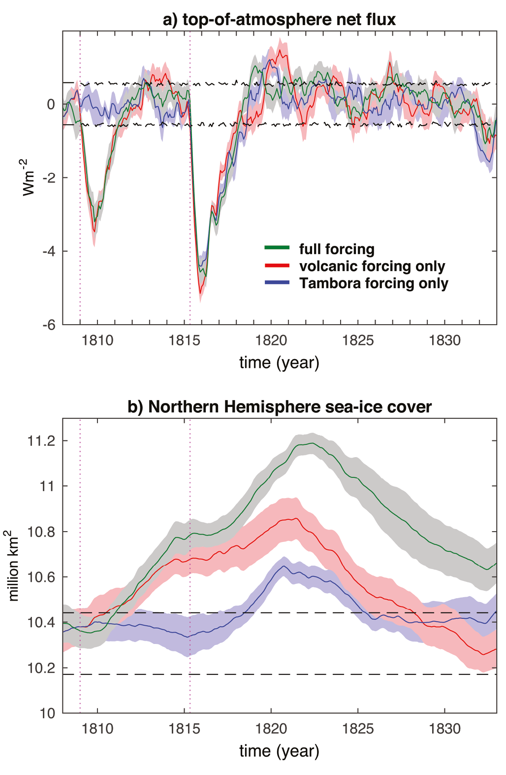 |
|
Figure 1: Simulated global-average top-of-atmosphere net radiative anomalies (a: 3-month smoothing) and simulated Arctic sea ice cover evolution (b: 61-month smoothing) around the 1815 Tambora eruption in three climate simulation ensembles with the ECHAM5/MPIOM coupled climate model, differing in the ensemble-mean initial state and in the applied forcing. Dark green: full-forcing conditions (including the Dalton Minimum of solar activity); Red: volcanic forcing-only conditions, including both the 1809 and 1815 eruptions; Blue: volcanic forcing-only conditions, without the 1809 eruption. Lines (shading): mean (1-σ standard error of the mean). Black dashed lines: 5th–95th percentile intervals for signal occurrence in the control run. Vertical dotted lines indicate the 1809 and Tambora eruptions. Each ensemble consists of 10 simulations differing in the initial state. Note that the Arctic sea ice response is significantly different in the three ensembles whereas the applied forcing, in terms of anomalous top-of-atmosphere net flux, is practically indistinguishable. For details see: Zanchettin et al. (2013a). |
Strong volcanic eruptions inject into the stratosphere massive amounts of chemically and microphysically active gases that lead to the formation of aerosol particles, affecting the Earth’s radiative balance and climate (Robock, 2000; Timmreck, 2012; LeGrande et al., 2016). Sulfate aerosol particles scatter solar radiation back to space, which results in global surface cooling and slowdown of the global hydrological cycle. The particles also absorb radiation in the infrared and near-infrared bands, causing local warming of the lower stratosphere. Both direct radiative forcing effects are temporary, their time scale being set by the persistence of the volcanic aerosol cloud in the lower stratosphere. This amounts to a couple of years in the case of the strongest recent tropical eruptions, such as the 1815 eruption of Mt Tambora in Indonesia (Fig. 1a). However, the climatic impact of strong volcanic eruptions can last well beyond the timescale of the direct radiative perturbation through the dynamic alterations it induces in the entire coupled climate system. These include “feedbacks” in their classic definition of amplification and dampening loops related to changes in climatic variables that operate through changes in global-mean surface temperature (Boucher et al., 2013). For instance, the so-called “polar amplification” of climate signals – mainly a consequence of positive feedbacks involving snow cover and sea ice – provides one element of inter-hemispheric asymmetry to the decadal climate response to volcanic eruptions through global radiative cooling (Zanchettin et al., 2014). Dynamical impacts further stem from the spatially heterogeneous structure of volcanic forcing.
In the case of tropical eruptions, for which the bulk of the volcanic aerosol cloud remains largely constrained in the tropical stratosphere, simple theoretical arguments indicate that the aerosol radiative heating enhances the upper-level equator-to-pole temperature gradients that, by thermal wind balance, can force a strengthened stratospheric polar vortex in both hemispheres, as diagnosed from climate models (e.g., Stenchikov et al., 2002; Zanchettin et al., 2014). The consequent downward penetration of the westerly wind anomalies at the edge of the polar vortex and their interaction with topography provide further elements of a top-down atmospheric mechanism of volcanic forcing. In the Northern Hemisphere, its tropospheric effects during the first post-eruption winter typically project on a positive anomaly of the North Atlantic Oscillation/Arctic Oscillation (NAO/AO) and associated continental warming (Stenchikov et al., 2006; Graf et al., 2014; Zambri and Robock, 2016). This is a key component of a major recognized general pathway of volcanically-forced decadal climate signals (Otterå et al., 2010; Zanchettin et al., 2012).
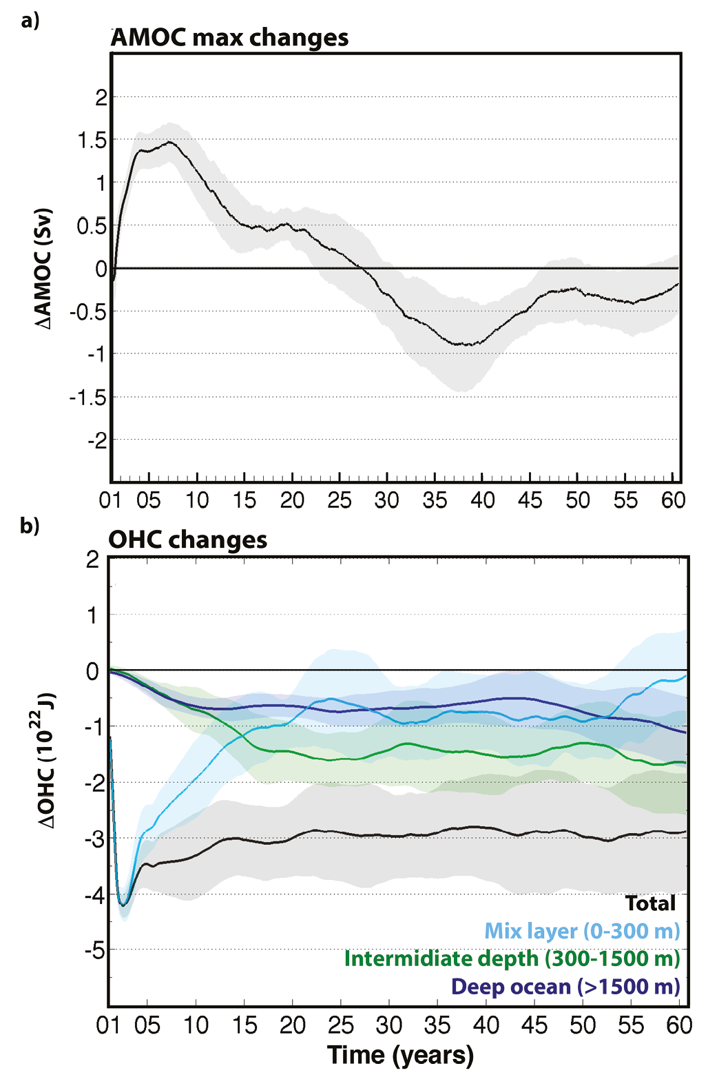 |
|
Figure 2: Decadal oceanic response to a high-latitude eruption resembling the multistage 1783 eruption of Laki (Iceland) simulate by the NorESM coupled climate model. a) Changes in the strength of the Atlantic Meridional Overturning Circulation (AMOC) estimated as the maximum of the zonally-integrated overturning stream function in the Atlantic. b) Changes in Ocean Heat Content (OHC) averaged from the surface to selected depths for the global ocean. In both panels the solid lines denote the ensemble average changes and shadings represent the confidence intervals at approximate 95% level (twice the standard error of the mean) of the difference in all pairs of experiments that comprise the ensembles. The ensemble consists of 10 simulations differing for the initial state. Anomalies are calculated with respect to a control simulation. The figure has been adapted from Pausata et al. (2015). |
Specifically, the NAO-related post-eruption modifications to the wind field modify the circulation in the upper North Atlantic Ocean and locally enhance oceanic convective mixing through anomalous turbulent heat and freshwater fluxes. These superpose on the extensive buoyancy effects of the post-eruption radiative cooling, leading to strengthened deep water formation. The slow propagation of so-formed water masses in the ocean abyss is expected to protract the fast oceanic response to decadal time scales through the tendency for reinvigoration of the oceanic meridional overturning circulation that culminates several years – up to a decade or so – after major eruptions, as diagnosed from models. Implications for meridional ocean heat transports and sea ice dynamics contribute to regional characterization of the signal, and hence to recognizable traces of volcanic signals especially in extratropical and polar regional climates (Zanchettin et al., 2012, 2013b; Sicre et al., 2013). Lacking further external excitation (e.g., by a successive eruption), negative feedbacks eventually become predominant and the near-surface system relaxes back to the mean pre-eruption state as part of a roughly bi-decadal fluctuation. The feedback loop thus sets the phase of internal modes of interdecadal climate variability (Otterå et al., 2010), whose effects can be protracted, with dampening intensity, beyond one fluctuation (Swingedouw et al., 2015). In the latter case, deep ocean anomalies may remain significant for much longer (Gleckler et al., 2006; Gregory, 2010). A similar interdecadal general oceanic response is also found for high-latitude eruptions, for which it is the direct radiative surface cooling at subpolar latitudes linked to the confinement of the volcanic aerosol cloud to the eruption’s hemisphere that typically leads to enhanced oceanic deep convection (Fig. 2, see also Pausata et al., 2015).
Knowledge gaps
The general framework outlined above is useful to identify the core dynamics involved in post-eruption decadal climate variability. However, several caveats must be taken into consideration. Above of all, direct observations of strong volcanic eruptions are very few - only five in the instrumental period - which does not allow robust statistics of their climate impact, and hence attribution. Therefore, large part of our knowledge builds on climate model simulations and proxy-based climate reconstructions, both of which have large uncertainties and deficiencies (e.g., Zanchettin, 2017). Incessant improvement in both tools brings old evidence back into the discussion. For instance, the mechanisms leading to a preferred enhanced stratospheric polar vortex in post-eruption winters have been questioned by recent studies suggesting that the mechanism based on the thermal wind balance and outlined above does not always hold (e.g., Bittner et al., 2016), possibly as the zonal wind response to direct aerosol radiative heating may be dominated by other effects, such as the residual circulation response to anomalous wave activity (Toohey et al., 2014).
Accordingly, obvious implications for the polar vortex response stem from the tropical Pacific, a known critical source of tropospheric wave disturbances affecting stratospheric dynamics (e.g., Graf et al., 2014). Instrumental observations and climate proxy-based reconstructions indicate that volcanic eruptions tend to be followed by an El Niño event. A newly discovered causal mechanism is initiated by cooling over Africa (the largest tropical landmass), which reduces precipitation and forces an atmospheric Kelvin wave response that couples with western Pacific convection to trigger westerly wind anomalies and a Pacific El Niño. While modulated by the seasonal cycle of convection, the effect of volcanism onwind forcing over the Pacific persists during the year after the eruption, implying that the Pacific El Niño-like response involves more external forcing than traditional, internally generated events (Khodri et al., 2017). However, there are stratospheric (e.g., Scaife et al., 2009) and tropospheric (e.g., Graf and Zanchettin, 2012) pathways of El Niño forcing on the atmospheric circulation over the North Atlantic that project on a negative NAO; this would counteract the NAO+ tendency above described. In addition, sampling issues in simulation ensembles (Lehner et al., 2016) and uncertainty linked to the eruption’s season (Stevenson et al., 2017) are recently proposed explanations for reconstructions-simulations discrepancies in the estimated post-eruption cooling.
This outlines the complexity of competing influences on the top-down mechanism of volcanic forcing, hence on the post-eruption positive NAO anomaly for moderate or small tropical eruptions, whose uncertainty cascades on the decadal oceanic response. Ocean dynamics simulated by coupled models are another major source of uncertainty to be understood considering the different time scales of simulated oceanic responses (Otterå et al., 2010; Mignot et al., 2011; Zanchettin et al., 2012). Furthermore, the fact that a climate model spontaneously generates bi-decadal variability in the overturning circulation strength seems to determine its excitability to the general response mechanism outlined above (Swingedouw et al., 2015).
Inherent sources of uncertainty
The climatic response to a given volcanic eruption is highly specific. First, the general response mechanism strongly depends on the characteristics of the forcing. An obvious determinant factor is the magnitude of the eruption, whose potential control can be, for instance, estimated looking at the sea ice response. For a very strong eruption, polar amplification of the global cooling signal may lead sea ice to cover regions of strong oceanic deep convection, thereby hampering deep water formation through insulation of the ocean-atmosphere boundary. Associated increased freshwater export from the Arctic also contributes to stabilize the ocean water column. These will lead ultimately to a tendency for weakening – instead of strengthening – of the thermohaline circulation (e.g., Zhong et al., 2010; Mignot et al., 2011). Second, the way the volcanic aerosol cloud distributes in the stratosphere influences both the direct radiative and dynamic atmospheric responses (e.g., Toohey et al., 2014; Colose et al., 2016). In this regard, the latitudinal position of the erupting volcano is an obvious determinant factor, but similar uncertainty on the spatial structure of the volcanic aerosol cloud can be originated by the season of the eruption (Stevenson et al., 2017).
A milestone in our understanding of volcanically forced decadal climate variability was the recent recognition that the mean climate state, the phase and amplitude of ongoing internal variability at the time of an eruption, such as that associated with major climatic modes including, e.g., El Niño Southern Oscillation (ENSO) or the Quasi-Biennial Oscillation (QBO), and the presence of additional forcing factors crucially determine how the climate system responds to the volcanic forcing (Zhong et al., 2010; Zanchettin et al., 2012, 2013a; Berdahl and Robock, 2013; Swingedouw et al., 2015; Pausata et al., 2016). Fig. 1 (after Zanchettin et al., 2013a) shows the role of background conditions for the case of Arctic sea ice response to the 1815 Tambora eruption simulated in three ensembles in which the volcanic forcing is the same but background climate state and histories are different. Results show that a significant increase in Arctic sea ice cover is consistently diagnosed after the eruption in all ensembles but the average anomalies differ in both magnitude and duration. The inter-ensemble differences in the Arctic sea ice response reflect substantial differences in the decadal feedback mechanisms activated in the coupled atmosphere-ocean-sea-ice system after the eruption.
This dependency on the background climate state can partly explain the different, often contrasting, results found for simulated and reconstructed post-eruption decadal variability from different volcanic eruptions (Zanchettin et al., 2013a,b). This concept also allows understanding how the timing between subsequent volcanic eruptions can deterministically influence the response in the case of a volcanic cluster. Specifically, if two eruptions are roughly paced at one period of the above-mentioned decadal mechanism (roughly two decades), they will interfere constructively, as they will occur around the same phase of internal modes of oceanic variability. In contrast, if they are paced at half the period of the mechanism (a decade or so), they will interfere destructively (Swingedouw et al., 2015). Intriguingly, both cases apply to the most recent strong volcanic eruptions: Agung in 1963 and El Chichón in 1982 are paced at roughly two decades (constructive interference), while El Chichón and Pinatubo in 1991 were paced at roughly one decade (destructive interference). This finding widens margins for long-term predictability of decadal climate impacts by strong volcanic eruptions.
Opportunities for progress
A series of research initiatives are currently contributing to building the scientific basis for reaching such an ambitious objective by filling major gaps of understanding. A first goal of current research is robust characterization, by means of climate models with interactive stratospheric aerosols, of the forcing generated by a given eruption based on the estimated amount of gaseous sulphur species it injects in the stratosphere. The WCRP/SPARC Stratospheric Sulfur and its Role in Climate (SSiRC) initiative (http://sparc-ssirc.org/ssirc.html, Timmreck et al., 2016b) coordinates the international activities on stratospheric aerosol research aiming at better understanding and hence modeling of the stratospheric aerosol layers and their controls. SSiRC will help study why the characterization of the volcanic aerosol cloud and the radiative forcing generated by state-of-the-art global aerosol models for a certain sulphur injection remain highly uncertain (e.g., SPARC, 2006; Zanchettin et al., 2016). Focus will be in particular on model inconsistencies related to the treatment of aerosol microphysics and climate physical processes, such as stratospheric circulation and stratosphere-troposphere coupling.
In addition, unpredictability of timing and magnitude of volcanic eruptions is a major source of uncertainty and the climate community should be prepared for such an eventuality. Therefore, a new SSiRC initiative called VolRes ("Volcano Response Plan after the next major eruption") has been launched aiming at developing a scientific plan to prepare observational and modelling tools and strategies to be readily applied for the next major volcanic eruption. Characterization of the potential climatic impact of an eruption in the more distant future (such as envisaged for end-of-the-century warming scenarios) bears additional uncertainties related to the dependence of dynamics of the eruption plume on the atmospheric stratification and tropopause height, in turn subject to global temperature changes (Aubry et al., 2016).
Finally, the “Model Intercomparison Project on the climatic response to Volcanic forcing” (VolMIP) (Zanchettin et al., 2016) has been created as part of the Coupled Model Intercomparison Project phase 6 (CMIP6), to define a coordinated protocol for idealized volcanic-perturbation experiments to improve comparability of results across different climate models. Interest is on various aspects of volcanically-forced climate variability, with specific sets of experiments designed to investigate both the seasonal-to-interannual atmospheric response and the interannual-to-decadal response of the coupled ocean-atmosphere-sea-ice system. Through systematic and consistent (across the different models) sampling of internal variability (e.g., ENSO, QBO), VolMIP will allow the identification of robust response mechanisms to volcanic forcing or explain the lack thereof.
VolMIP will also foster investigation of simulated Southern Hemispheric responses to volcanic forcing, currently an overlooked topic due to the known severe climate model biases in the Southern Hemisphere (e.g., Simpson et al., 2012; Salleé et al., 2013; Turner et al., 2013). More generally, if volcanically-forced decadal climate variability can be understood through the excitation by volcanic forcing of internal modes of climate variability, confidence must be built on the accurate and robust simulation of such modes. Current climate models, however, have difficulties in reproducing the observed spatial pattern, time scales and teleconnections of dominant modes such as ENSO (e.g., Zou et al., 2014) or the Atlantic Multidecadal Oscillation (Kavvada et al., 2013).
Only a few studies specifically focused on the quantitative assessment of volcanic forcing impacts on decadal climate predictions and potential predictability (Collins, 2003; Shiogama et al., 2010; Timmreck et al., 2016a). Overall, in the presence of strong natural climate variability on the one hand and because of different magnitude and frequency of volcanic eruptions on the other hand, it is difficult to assess the potential predictability from volcanoes of regional climates. Improvements of decadal climate prediction systems concerning implementationof volcanic forcing (e.g., LeGrande et al., 2016) and bias estimation and correction (e.g., Hawkins et al., 2014) are milestones toward robust prediction of volcanically-forced decadal climate variability. Along this long-term goal, within CMIP6, a joint decadal climate prediction experiment between VolMIP and the Decadal Climate Prediction Panel (Boer et al., 2016) will be conducted to address the climatic implications if a Pinatubo-like eruption would have occurred in 2015.
In conclusion, there is emerging evidence that volcanic forcing can significantly affect decadal climate variability through mechanisms that are increasingly better understood. Milestones on the road toward robust prediction of volcanically-forced decadal variability include improved understanding and implementation of aerosol forcing in decadal prediction systems and improved simulated representation and estimation of internal decadal climate variability.
affiliations
1 Department of Environmental Sciences, Informatics and Statistics, University Ca’Foscari of Venice, Italy
2 Department of Meteorology (MISU), Stockholm University, Sweden
3 Department of Earth and Atmospheric Sciences, University of Quebec in Montreal (UQÀM), Montreal (QC), Canada
4 IRD/IPSL/Laboratoire d'Océanographie et du Climat, Paris, France
5 Max Planck Institute for Meteorology, Hamburg, Germany
6 University of Cambridge, Cambridge, UK
7 Department of Environmental Sciences, Rutgers University, New Brunswick, USA
8 Met Office Hadley Centre, Exeter, UK
references
Robock, A., 2000: Volcanic eruptions and climate, Rev. Geophys., 38, 2: 191-219
Richard P. Allan
Introduction
The Earth’s energy balance represents a nexus between radiative forcings which set the trajectory of climate change and feedbacks which determine the nature and magnitude of the response. Yet entwined within the observed decadal variability and trends are complex, unforced interactions within the climate system. The energy and water cycles are intimately linked and observed precipitation changes contain signals from unforced fluctuations as well as rapid adjustments to radiative forcing and responses to the longer-term heating or cooling; this is mediated by the oceans which dominate the effective heat capacity of the climate system. It is essential to monitor key indicators of climate including the evolving energy budget to interpret global change in the context of intrinsic multidecadal variability.
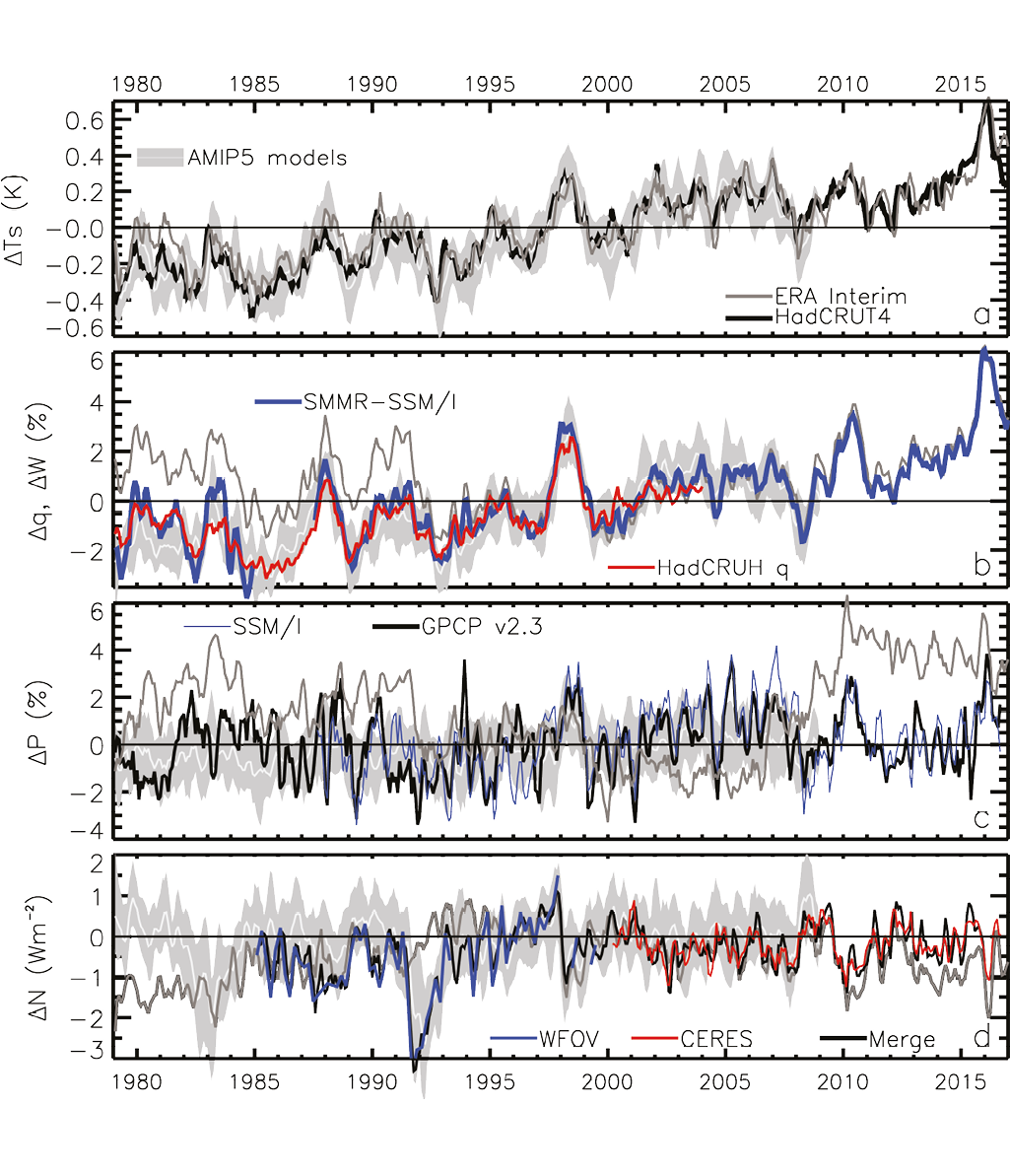 |
|
Figure 1: Deseasonalised monthly anomalies with respect to 1995-2000 in global mean (a) surface temperature, (b) column integrated or surface water vapor, (c) precipitation and (d) top of atmosphere net radiation for a combination of satellite and surface observationally based estimates, atmosphere-only climate models using prescribed observed sea surface temperature and sea ice (AMIP) and a the ERAI reanalysis over the period 1979-2016 (3 month smoothing is applied). |
Fig. 1 displays variability and change in global-mean surface temperature, atmospheric moisture, precipitation and the top of atmosphere energy balance over the period 1979-2016. This includes a mixture of observationally-based estimates combined with the European Centre for Medium-range Weather Forecasts (ECMWF) interim reanalysis (ERAI) (Dee et al., 2011), which continually adjusts a numerical model by applying data assimilation to an evolving and diverse set of global observations. Also shown are atmosphere-only “AMIP” experiments from phase 5 of the Coupled Model Intercomparison Project (CMIP5) (Taylor et al., 2011) which apply realistic radiative forcing and observed surface temperature and sea ice distributions over the 1979-2008 period (an ensemble mean with a one standard deviation spread across models are displayed). The surface temperature, water vapor and precipitation variability depicted in Fig. 1a-c update Allan et al. (2014a) while Fig. 1d exploits top of atmosphere energy budget estimates from Allan et al. (2014b).
Considering deseasonalised monthly surface temperature (Ts) anomalies from HadCRUTv4.5 (Morice et al., 2012), the globe has warmed at 0.16 K/decade when considering the period 1988-2015 chosen to coincide with the introduction of the special sensor microwave imager (SSM/I) series of satellite instruments in 1987.
This trend is punctuated by episodic warm El Niño events (e.g. 1997/98, 2015/16) and cool La Niña episodes (e.g 1999, 2011) which alter global monthly mean surface temperature by up to around 0.2-0.3 K. At longer timescale, increased La Niña frequency linked to multi-decadal strengthening of the Walker circulation (L’Heureux et al., 2013) suppressed decadal surface warming rates during 2000-2010 (Xie & Kosaka, 2017). The opposite was observed during 1980-1990 characterized by recurrent and strong El Nino events, which boosted the warming trend. The Ts anomalies are well represented by AMIP simulations (which prescribe observed sea surface temperatures while land Ts is explicitly simulated) and ERAI (which also prescribes ocean surface temperature but land Ts is somewhat constrained by observations through data assimilation). ERAI anomalies up to 0.2 K higher than HadCRUT4 in late 2016 are likely due in part to the lack of interpolation of observed values over the Arctic (Cowtan and Way, 2014).
Atmospheric column integrated water vapour closely tracks the temperature changes, as expected from the strong temperature dependence of saturation vapor pressure determined by the Clausius Clapeyron equation, and there is broad agreement between the range of surface in situ observations, satellite-based datasets and AMIP simulations. The satellite estimates sample the ice-free ocean (a combination of microwave measurements taken from the F08/F11/F13/F17 series of Defence Meteorological Satellite Program satellites; Wentz, 2013) and are here combined with ERAI over remaining regions: these indicate a moistening of 1.2 %/decade for 1988-2015; interestingly this trend is only marginally suppressed (by about -0.2 %/decade) during the 2000-2012 period of slower surface warming.
The resultant additional water vapor continuum absorption in the more transparent window regions of the infrared spectrum cause a reduction in surface loss of clear-sky longwave radiation of ~1.4 Wm2 per mm of precipitable water vapor (Allan, 2009) which translates to reduced clear-sky surface net longwave radiative loss of ~0.4 Wm2 per decade, consistent with more detailed modelling estimates (Wild et al., 2008). Enhanced absorption of sunlight by the increasing water vapor additionally reduces net radiative energy loss by the atmosphere and contributes to solar “dimming” at the surface (Haywood et al., 2011).
Observed global mean column integrated moisture increases with Ts at 7.2±0.4 %/K based on linear regression (r = 0.87), in agreement with the combination of Ts and moisture trends. This is consistent with simple thermodynamics which strongly determine global low altitude water vapor although variability and change over land appears less constrained (Simmons et al. 2010). Climate model AMIP simulations capture the SSM/I-based variability and earlier Scanning Multi-channel Microwave Radiometer (SMMR)-based microwave estimates while ERAI anomalies are in close agreement after the 1991-1993 period during which an unrealistic drop in global ocean moisture affects the reanalysis. There is a remarkable agreement in interannual variability between independent HadCRUH surface specific humidity observations (Willett et al., 2008) and the satellite-based estimates of column integrated moisture, with a consistent increasing trend over the coinciding 1988-2004 period (Allan et al., 2014a).
Low altitude moisture provides the fuel for rainfall events (Trenberth et al., 2003) yet global precipitation is determined by atmospheric energy balance, primarily attributable to net radiative energy loss (Allen and Ingram, 2002; O’Gorman et al., 2012). Given these global driving factors, combined with the heterogeneous distribution of precipitation and associated measurement limitations, it is no surprise that variability and trends in global precipitation (Fig. 1c) contrast markedly to that of water vapor and temperature (Fig. 1a-b). Global mean precipitation from the Global Precipitation Climatology Project (GPCP v2.3; Adler et al., 2017), a combination of satellite-based and land surface gauge-based estimates, appears to display greater month to month variability compared to longer time-scale changes than temperature or water vapor; co-variability with these variables and similarity to AMIP5 simulations appears less coherent (Fig. 1c) with barely significant global precipitation trends during 1988-2015 (0.3 %/decade; r=0.19) and no significant trend during the period of slower surface warming 2000-2012, consistent with understanding of radiative forcing and precipitation response (Allan et al., 2014a; Saltzmann, 2016).
It is reassuring but no surprise that SSM/I-based estimates agree with GPCP since SSM/I data over the ice-free ocean is used in the generation of GPCP estimates while over other regions data is identical in this merged estimate. However, the changing observing system seriously compromises the global precipitation variability depicted by ERAI as previously reported (Dee et al., 2011; Allan et al., 2014a). Interannual coupling of GPCP precipitation with HadCRUT Ts over this period is 3.0±0.7 %/K (r=0.37), consistent with estimates of temperature dependent precipitation sensitivity (Andrews et al., 2010; Myhre et al., 2017). Global precipitation increases with global Ts primarily due to the enhanced radiative loss for higher surface and atmospheric temperatures, set by the thermodynamics of the coupled system (Roderick et al. 2014; Myhre et al., 2017) although this is tempered by the additional absorption of sunlight by higher water vapor loadings (Allan 2009) and modified by sensible heat flux changes. However, apparent short-term increases of 2-3% in global precipitation during warm El Niño events (e.g. 2010 and 2016) coincide with increases in Ts of just 0.2-0.3 K, a much greater precipitation sensitivity than anticipated from energy budget considerations and indicative of a subtler influence of spatial reorganisation of circulation systems and energy in the climate system.
Variability in net downward top of atmosphere radiation imbalance by satellites are generally well captured by the AMIP5 simulations (Allan et al., 2014b) indicating that radiative forcing and feedback response are well simulated when realistic ocean surface temperature is prescribed. ERAI also captures month to month variability in the radiation budget remarkably well given that cloud cover, which dominates these fluctuations, is not directly assimilated. However, decadal variability and trends are unrealistic and the reanalysis does not represent volcanic radiative forcing as evident from the lack of response to the 1991 Pinatubo eruption. Variability is dominated by cooling following the Pinatubo volcanic eruption in 1991 (up to -3 Wm2 caused by the reflective volcanic aerosol haze in the stratosphere) and El Niño events in which a warmer atmosphere loses more energy to space through infrared emission. This reduced energy uptake is of order 1 Wm2 although an increase in energy uptake of about 0.2 Wm2 can occur as El Niño builds (Johnson and Birnbaum, 2017) and substantial reorganisation of energy in the upper 400m of the ocean occurs (Roemmich et al., 2015).
Recent estimates of net radiative imbalance at the top of the atmosphere of 0.6-0.8 Wm-2 for 2005-2015 (Johnson et al., 2016) are primarily determined by ocean heat content changes measured by Argo buoys; this and additional observations and assumptions are applied in anchoring the satellite records (Loeb et al., 2012) which themselves provide excellent representation of interannual variability and decadal trends. The net imbalance is remarkably stable over time with trends of just 0.02±0.01 Wm2 per decade over the period 1988-2015, substantially smaller than the expected uncertainty. This stability indicates no hiatus in anthropogenic radiative forcing despite slower global surface warming at the beginning of the 21st century (Xie & Kosaka, 2017) although there is intriguing evidence of distinct global energy budget response to Ts that influences interannual fluctuations, internal decadal variability and long-term climate response (Brown et al., 2014; Xie et al., 2015).
Ongoing monitoring of Earth’s energy budget and other key climate indicators combining a range of observations, reanalyses and model simulations is valuable for (i) detecting unrealistic behaviour in observing systems, (ii) identifying unusual or significant climate fluctuations and trends and (iii) improving understanding of physical processes and feedbacks. Isolating internally generated interannual to decadal variability from longer term climate responses is essential for interpreting changes in the global water cycle (Gu et al., 2016; Sukhatme and Venugopal, 2017) and the fundamental driving factors involving Earth’s energy balance (Palmer and McNeall, 2014; Trenbeth et al., 2016). This variability can potentially be exploited in elucidating regional feedbacks on internal decadal variability (Brown et al., 2014; Zhou et al., 2016; Xie et al., 2015) as well as in advancing understanding of how the spatial nature of climate change influences how sensitive the global climate is to radiative forcings (Gregory and Andrews, 2016).
The regional manifestation of changes in the energy budget and water cycle have been identified globally (Myhre et al., 2017; Bony et al., 2013) and at hemispheric (Hwang et al., 2013; Loeb et al., 2016; Stephens et al., 2017) to continental scales (Bollasina et al., 2011; Dong and Sutton, 2015). Applying a regional energy budget perspective is informative in understanding these water cycle responses (Muller and O’Gorman, 2011) and for tracking energy within the climate system: combining satellite radiation budget measurements with reanalysis energy transports to estimate surface fluxes can be used to identify regional decadal patterns of ocean heating (Liu et al., 2017) and potentially constrain ocean energy transports (Trenberth and Fasullo, 2017) and their changes from one decade to the next. These advances take observing systems and climate models to their limits (Desbruyères et al., 2016; Palmer, 2017; Wild, 2017). To further constrain long-term regional climate change responses to radiative forcings it is necessary to disentangle the distinct energy budget responses and feedbacks influencing internal decadal variability of the climate system.
affiliation
Department of Meteorology, University of Reading, UK
acknowledgements
Support was provided from the UK National Centre for Earth Observation (NCEO) and National Centre for Atmospheric Science (NCAS) and the Natural Environment Research Council SMURPHS (NE/N006054/1) and DEEP-C (NE/K005480/1) projects. The World Climate Research Programme's Working Group on Coupled Modelling is acknowledged for developing the CMIP model archive, and we thank the climate modelling groups for producing and making available their model outputs; for CMIP, the U.S. Department of Energy's PCMDI provided coordinating support and led development of software infrastructure in partnership with the Global Organization for Earth System Science Portals. AMIP5 climate model data sets were extracted from the British Atmospheric Data Centre (http://badc.nerc.ac.uk/home) and the Program for Climate Model Diagnosis and Intercomparison (https://pcmdi.llnl.gov/index.html). GPCP v2.3 data were extracted from http://gpcp.umd.edu. Merged radiation budget data (v3) are available from http://www.met.reading.ac.uk/~sgs02rpa/research/DEEP-C/GRL/ and CERES EBAF v2.8 and ERBS wide field of view (WFOV) v3 data was provided by the NASA Langley research centre. SSM/I and SSMIS v7 products were also obtained online (ftp.ssmi.com). HadCRUT4 data is available from http://www.metoffice.gov.uk/hadobs/hadcrut4/.
references
Adler et al. (2017) An Update (Version 2.3) of the GPCP Monthly Analysis (in preparation).
Gu, G., Adler, R.F. & Huffman, G.J. Clim Dyn (2016) 46: 1091. doi:10.1007/s00382-015-2634-x.
Dirk Notz
Introduction
The large-scale loss of Arctic sea ice in recent decades is one of the most prominent indicators of the ongoing global climate change. This derives from three main reasons. First, climate change is amplified in the Arctic (“Arctic amplification”, e.g. Pithan et al. (2013)), so consequences of changes in the global-mean climate are more readily observed at high latitudes compared to middle and lower latitudes. Second, while many observables change gradually with global mean climate, Arctic sea ice is among those observables that might eventually cross a binary threshold from “existing” to “non-existing”, which amplifies the perception of the underlying gradual trend. And third, as a consequence, changes in “Arctic sea ice coverage” are easier to grasp and communicate to a general public than changes in more abstract metrics such as “global mean temperature”.
The observed changes in Arctic sea ice are not only a clear local indicator of large-scale climate change; the ice loss also has a number of sometimes far-reaching worldwide consequences. These include physical phenomena such as the possible impact on mid-latitude weather system or the disruption of the oceanic uptake of CO2, but also societal consequences such as the opening of new shipping routes or the necessary changes in the livelihood of the Arctic indigenous population.
The importance of sea ice loss both as an indicator and as an active player in the ongoing climate change has motivated some intense research into understanding the temporal evolution of sea ice on time scales from seasons to decades. In this contribution, I use a combined analysis of the observational record and of climate model simulations to explain and summarize some of these findings.
Seasonal variability: The importance of atmospheric chaos
Recent years have seen an increase in research activities aimed at forecasting the evolution of Arctic sea ice on time scales of a few months. There is good reason to believe that such seasonal-scale forecasts should be possible, with model studies emphasizing in particular the rather long memory of the sea ice state imprinted in the sea ice thickness fields (e.g., Blanchard-Wrigglesworth et al., 2011), and the long memory of the oceanic heat content that determines the regional evolution of Arctic sea ice (e.g., Bushuk et al., 2015).
The underlying research is in part driven by very practical applications, such as ship routing, but will also increase our fundamental understanding of air–ice–sea interactions at high latitudes. Related activities are for example coordinated by the Polar Prediction Project with its flagship Year of Polar Prediction 2017-2019 (www.polarprediction.net, under the auspices of WMO World Weather Research Programm WWRP), by the Polar Climate Predictability Initiative (www.climate-cryosphere.org/wcrp/pcpi, under the auspices of the WMO World Climate Research Program WCRP), and by the Sea ice Prediction Network with its Sea ice Outlook activity (www.arcus.org/sipn).
In this latter activity, various research groups try to forecast the minimum Arctic sea ice area coverage in September based on the observed state of the sea ice cover from May onwards. The groups use a variety of methods, ranging from heuristic methods to seasonal prediction systems based on coupled climate models. An analysis of the forecast quality of the various methods has shown a mixed picture, with no single method giving significantly better results than any other (Stroeve et al., 2014).
This finding is possibly surprising in that idealised studies with seasonal prediction systems usually result in significant prediction skill of many months up to a few years in advance (Blanchard-Wrigglesworth et al., 2016). In this framework referred to as “perfect model”, a single model simulation is taken as the “observed truth”, while additional model simulations with slightly perturbed initial conditions are used to estimate whether this “truth” can be forecast.
The striking difference in the forecast quality of such idealised studies compared to those trying to forecast the real world might be explicable by three main factors. First, the forecast skill strongly depends on a proper knowledge of the initial state of the system. As shown by Bunzel et al. (2016), the incomplete knowledge of May sea ice concentration as reflected by the differences between different satellite data sets can cause differences in forecast mean September Arctic temperature of several degrees, and in forecast September Arctic sea ice area of 2 million km2. The incomplete knowledge of initial conditions of the sea ice cover arises because the microwave signature that is usually used to assess ice concentration reacts sensitively to snow coverage and melt-pond formation on the ice, for example. Different algorithms compensate these uncertainties in different ways, causing substantial differences of the observed sea ice area. Because of positive feedbacks such as the ice-albedo feedback, these differences in initial conditions are substantially amplified during summer and contribute to the much lower forecast quality of real-world applications compared to perfect model studies. Incomplete knowledge of the state of the underlying ocean certainly also contributes to these uncertainties.
Second, the forecast skill might be negatively affected by the initial shock and drift in the forecast runs in a real-world application. Both are absent in a perfect-model study, as its forecasts are usually started from a model state that is perfectly consistent with model physics. In contrast, the initial state for any simulation starting from a model state based on observations will usually be more or less inconsistent with model physics, possibly causing substantial drift that can quickly compensate for any added value from the assimilation of observations.
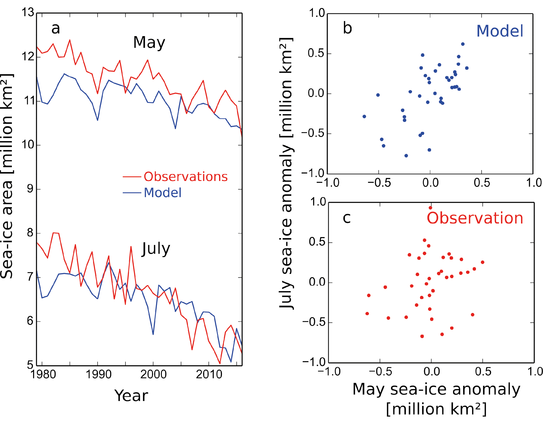 |
|
Figure 1: (a) Evolution of modeled and observed Arctic sea ice area in May and July (1979–2016. (b) Modeled Arctic sea ice area in July as a function of observed Arctic sea ice area in May of the same year. (c) Observed Arctic sea ice area in July as a function of observed Arctic sea ice area in May of the same year. Observations for all panels are based on the Arctic sea ice index (Fetterer et al., 2002, updated 2016). Model simulations for all panels are based on the first ensemble member of the CMIP5 simulations of MPI-ESM-LR (Notz et al., 2013). |
A third factor that might cause the systematically better forecast skill in idealised model studies relates to possible model errors in the simulation of the persistence of the Arctic sea ice cover. Take, for example, the relationship between Arctic sea ice area in May and Arctic sea ice area in July during the observational period 1979–2016 (Fig. 1a). The time series of these two months are highly correlated because of their underlying trend, both in the observations and in the model simulations.
However, the detrended time series are only significantly correlated in the model simulations (Fig. 1b), with the Pearson rank coefficient of the correlations indicating a chance of far less than 1 % that these time series are uncorrelated. In contrast, chances are above 30 % that there is no significant correlation between the detrended observed time series of sea ice area in May and the detrended observed time series of sea ice area in July (Fig. 1c).
This suggests that at least an idealised study based on the particular model employed here (MPI-ESM-LR) will result in an unrealistically large potential forecast skill of seasonal predictions. We are currently examining whether this finding also holds for other models, and are in particular trying to investigate the underlying reasons for this different behaviour in the model compared to reality.
Annual variability: The importance of negative feedbacks
In addition to seasonal forecasts on time scales of a few months, also forecasts on time scales of a few years have made some headlines over the past decade. These headlines were usually related to claims that the Arctic would lose its remaining summer sea ice within just a few years. The underlying reasoning of such claims was often related to a discussion of a possible ’tipping point’ that is related to the ice-albedo feedback. Given the substantial loss of Arctic sea ice in the past few years, the ocean could potentially absorb enough heat to rapidly melt the remainder of the sea ice cover.
However, our current understanding of the Arctic climate system strongly suggests that this reasoning is unrealistic. A first indication for this finding derived from model experiments in which all Arctic sea ice was synthetically removed from the Arctic Ocean at the onset of summer, thus maximising the possible ice-albedo feedback (Tietsche et al., 2011). Despite such maximised feedback, the ice cover recovered in these experiments within just a few years. This is because on annual time scales, negative feedbacks dominate the evolution of the Arctic sea ice cover. Three negative feedbacks are particularly important: First, the open ocean very effectively releases its heat to the atmosphere during winter, causing a rapid loss of much of the heat that was accumulated in the ice-free water during summer. Second, the thin ice that forms during winter can grow much more rapidly than ice that survived the summer, because heat can more effectively be transported from the ocean to the atmosphere when the ice cover is thin (Bitz and Roe, 2004). Third, as ice forms later in the season, it will carry a thinner insolating snow cover as any snow fall occurring before ice formation simply falls into the open ocean (Notz, 2009).
The effectiveness of these negative feedbacks on an annual time scale is not only apparent in our model simulations; the observed time series of Arctic summer sea ice also carries a clear signature of such mechanisms. A year with a strong drop in ice coverage during September is usually followed by an increase in September ice coverage in the following year. More formally, the time series shows significant negative autocorrelation (Notz and Marotzke, 2012). If indeed the ice albedo feedback was as effective on annual time scales as implied by statements supporting the entire loss of Arctic summer sea ice within this decade, one would certainly expect that any year with a strong drop in ice coverage would be followed by a year with yet another drop. This is found neither in the observational record, nor in model simulation. This underpins the dominance of negative feedbacks, which stabilize the Arctic ice cover and prevent a possible “tipping point”.
Decadal variability: The importance of internal variability
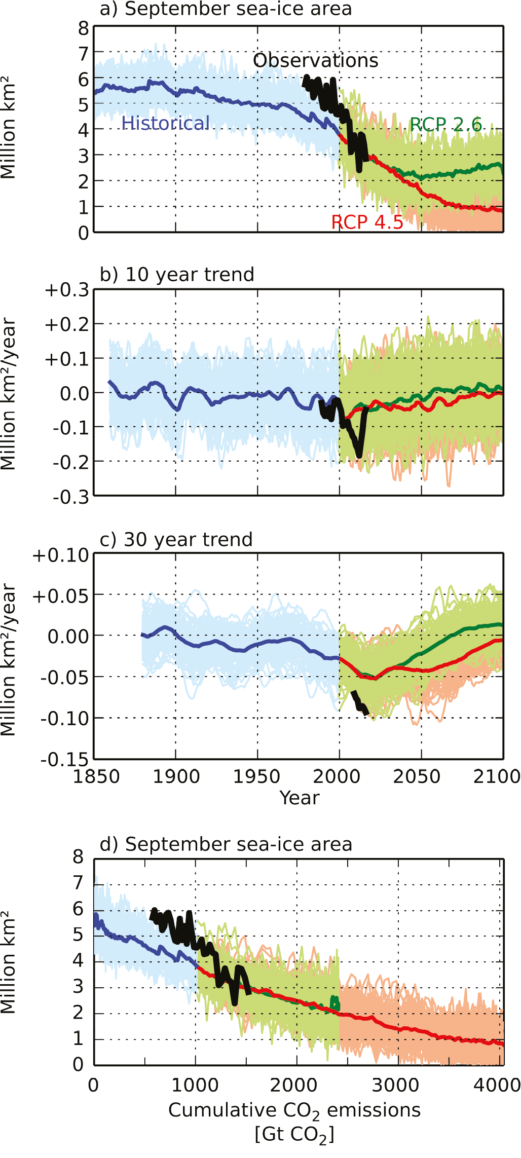 |
|
Figure 2: (a) Evolution of modeled and observed Arctic sea ice area in September (1850–2016). (b) Evolution of ten-year linear trends of Arctic sea ice area, plotted at the end point of the ten year averaging period. (c) Evolution of thirty-year linear trends of Arctic sea ice area, plotted at the end point of the thirty year averaging period. (d) Evolution of modeled and observed Arctic sea ice area in September (1850–2100) as a function of cumulative anthropogenic CO2 emissions. Observations for all panels are based on the Arctic sea ice index (Fetterer et al., 2002, updated 2016). Model simulations for all panels are based on the 100 member ensemble of MPI-ESM-LR. |
Internal climate variability not only governs a substantial part of the sea ice evolution on seasonal-to-interannual time scales as discussed above, but also affects the longer term trends of sea ice (Swart et al., 2015; Notz, 2015). To exemplify this, large ensembles of simulations of coupled Earth System Models are particularly helpful (Swart et al., 2015). At the Max-Planck-Institute for Meteorolgy, we have recently finished a 100 member large ensemble of simulations with our Earth System Model MPI-ESM-LR for the historical period, and for two possible future emission scenarios, RCP2.6 and RCP4.5. In comparing the simulated Area sea ice area during September with the observational record 1979–2016, we find that the observed sea ice area is at the upper edge of the ensemble spread during the earlier years of the record, and approaches the mean of the ensemble in the more recent past (Fig. 2a).
Ten-year long trends within the observational record have consistently been negative with values ranging from a mean loss of 23 000 km2 per year during the period 1990–1999 to a mean loss of 180 000 km2 during the period 2003–2012 (black line in Fig. 2b). This latter period includes the two record minima that have been observed in 2007 and 2012. For the most recent period 2007-2016, the average ice loss has been around 50 000 km2 per year. All these numbers are well within the range simulated by individual ensemble members of MPI-ESM-LR, which show over ten year-long periods a sea ice evolution ranging from a mean loss of around 200 000 km2 per year to a mean gain of around 100 000 km2 per year (shaded range in Fig. 2b). In particular, it is noteworthy that the mean ten-year long trends for the first 20 years of the satellite record and for the most recent past are very close to the mean trend of the 100 member ensemble, including a slowdown of the ice loss during the 1990s and an accelaration during the early 2000s. This agreement during substantial periods of the record suggests that the rather sudden drop in observed sea ice area that occurred in the year 2007 has been an extreme event compatible with internal climate variability and therefore cannot directly be compared to the ensemble mean across several models or to the ensemble mean across multiple simulations with one model. If this characterisation of this sea ice loss as an extreme event was correct, any realistic climate model should on average simulate a slower ice loss than has been observed (see also Notz (2015) for a detailed discussion).
Regarding the future evolution of sea ice, the model simulations with MPI-ESM-LR suggest a similar range of possible ten year trends than over the past few decades. Hence, in extreme cases and providing the hypothesis that the level of internal climate variability simulated is correct, the sea ice cover might in the future potentially once again lose ice as fast as during the first decade of this century, or, in contrast, gain an average of 100 000 km2 per year for a decade despite the ongoing global warming (see also Swart et al., 2015).
In order to more confidently predict the near-term evolution of Arctic sea ice, the underlying reasons for internal variability must be understood better. A number of recent studies point in particular to the impact of oceanic heat transport into the Arctic for driving low-frequency variability of the ice cover, including a possible contribution to the recent acceleration of sea ice loss (e.g., Årthun et al., 2012). These studies emphasize that a scenario with a much slower sea ice loss for the next decade is plausible if oceanic heat transport were to weaken (Zhang, 2015; Yeager et al., 2015). Such weakening of the oceanic heat transport would not only affect the sea ice cover itself, but also its future predictability on seasonal time scales (Germe et al., 2014). This then directly links the challenge of decadal forecasting of sea ice to that of its seasonal forecasting as described in the previous section.
Long-term changes: The importance of the external forcing
On longer time scales, internal variability also remains a substantial contributor to the evolution of Arctic sea ice area. The 100 member simulations suggest a possible spread in observed September sea ice area of around 2 million km2 for any given year (Fig. 2a). In terms of trends, even long-term trends over 30 years show substantial variability (Fig. 2c). For example, the model suggests that over the past 30 years, sea ice area in the Arctic could have remained roughly constant or could have decreased roughly as quickly as observed. This large spread in 30-year long trends again suggests that using these trends as metrics for the purpose of model evaluation can be misleading (Notz, 2015), in particular if the observed evolution of Arctic sea ice corresponds to a possible extreme event.
Despite the large impact of internal variability, the dominant role of external forcing in the observed evolution of Arctic sea ice is clear (Notz and Marotzke, 2012). The weight of the external forcing becomes particularly apparent if one examines the average evolution of Arctic sea ice coverage in the 100 member ensemble as a function of cumulative anthropogenic CO2 emissions (Fig. 2d). The long-term evolution of the sea ice cover directly follows the cumulative emissions. In particular, there is no clear difference in mean sea ice coverage between RCP 2.6 and RCP 4.5 for any given cumulative CO2 emission.
We have recently been able to explain this relationship, which is largely based on the fact that the position of the outer edge of the sea ice cover is determined by the net local energy balance (Notz and Stroeve, 2016). Any rise in atmospheric CO2 concentration increases the incoming longwave radiation at the ice edge, causing the latter to move northward to a region with less incoming shortwave radiation. For geometric reasons, these combined processes lead to a roughly linear relationship between Arctic sea ice loss and anthropogenic CO2 emissions in the observational record and in all CMIP5 model simulations. In the observations, about 3 m2 of sea ice are lost per ton of CO2 emissions, while the models on average only simulate an ice loss of 1.7 m2 per ton of CO2 emissions.
The fact that the relationship between cumulative CO2 emissions and Arctic sea ice area is roughly linear strongly suggests a dominating role of the CO2 emissions for the evolution of sea ice area. However, other external drivers are also apparent, in particular in the mean across all simulations of our 100-member ensemble. Most striking are temporary increases in Arctic sea ice area following large volcanic eruptions during the historical period, most recently in 1991 after the Pinatubo eruption, in 1982 after the eruption of El Chichon and in 1963 after the eruption of Mount Agung (compare also Zanchettin et al., 2014). Because of the large internal variability and the relatively short-lived response, these eruptions are impossible to identify in the temporal evolution of individual simulations nor the observational record, but they apparently have contributed to a synthetic improvement of CMIP5 sea ice simulations relative to CMIP3 sea ice simulations (Rosenblum and Eisenman, 2016).
Conclusions
This short overview presents some recent work on the variability and long-term evolution of Arctic sea ice area. For space constraints, the focus was only on September sea ice coverage as this is the month with the strongest observed trends. The discussion can be summarized as follows:
- On seasonal time scales, atmospheric internal variability and its imprint on sea ice renders skillful predictions of September sea ice coverage more than two months in advance inherently difficult.
- On annual time scales, negative feedbacks stabilize the sea ice cover. There is no “tipping point” beyond which the loss of the remaining summer sea ice becomes unstoppable.
- On decadal time scales, internal climate variability can cause a substantial acceleration or temporary recovery of the sea ice cover that renders the evaluation of individual model simulations based on their short-term trends impossible.
- On longer time scales, internal variability causes a substantial spread in possible 30-year long trends supporting for the production of large model ensembles. Nevertheless, the impact of anthropognic forcing on the long-term sea ice evolution is clear, with an average loss of 3 m2 of September sea ice cover per metric ton of anthropogenic CO2 emission.
affiliation
Max Planck Institute for Meteorology, Hamburg, Germany
references