PAGES Magazine articles
Yohan Ruprich-Robert1, Rym Msadek2
Introduction
  |
|
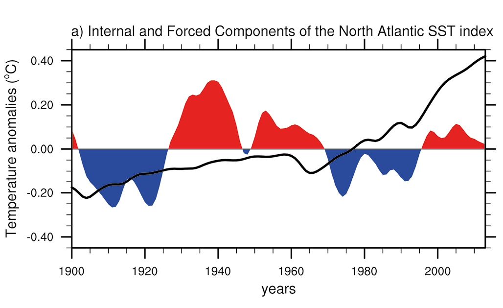
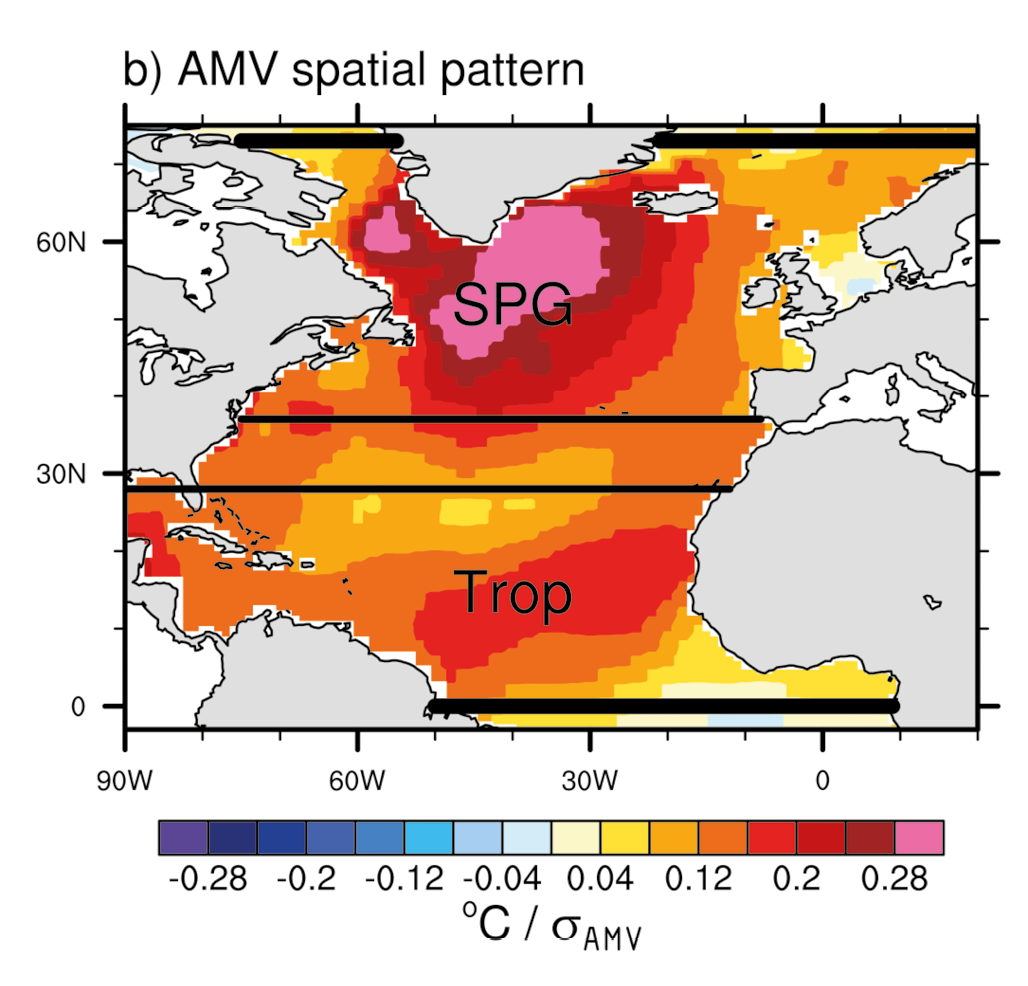
Figure 1: (a) Internal (red and blue) versus external (black) components of the observed North Atlantic SST multidecadal variability following Ting et al. (2009) definition. (b) Regression map of the observed annual mean SST (ERSSTv3; Smith et al. 2008) on the internal component of the North Atlantic SST index (i.e., the AMV index); units are oC per standard deviation of AMV index. Both SST field and AMV index time series have been low pass filtered prior to computing the regression, using a Lanczos filter (21 weights with a 10-yr cutoff period). The black latitudinal lines in b show the subpolar and tropical domains used for the SPG_AMV and Trop_AMV experiments (see section 2b). Figure from Ruprich-Robert et al. (2017). ©American Meteorological Society. Used with permission. |
During the last century, the observed annual mean North Atlantic sea surface temperatures (SSTs) exhibited multidecadal fluctuations superimposed onto a long-term warming trend. This multidecadal variability has been referred to as the Atlantic Multidecadal Oscillation (AMO) or Variability (AMV). The SST anomalies that define the AMV are characterized by a basin-scale anomalous pattern that has the same sign in the whole North Atlantic, and a maximum loading in the subpolar gyre (SPG) region (Fig. 1).
Previous studies have shown that the AMV is associated with, and possibly the source of, marked climate anomalies over many areas of the globe. This includes droughts over Africa and North America (Mohino et al., 2011; Enfield et al., 2001), decline in Arctic sea ice (Mahajan et al., 2011), changes in Atlantic tropical cyclone activity (Vimont and Kossin, 2007), and recently it has been linked with the global temperature hiatus (McGregor et al., 2014; Li et al., 2015). Additionally, due to its upstream location, the North Atlantic SST is a main actor of the European climate variability. Sutton and Hodson (2005) and Sutton and Dong (2012) argue for the existence of a causal link between the warm phase of the AMV and warmer conditions than normal over Central Europe, drier conditions over the Mediterranean basin, and wetter conditions over Northern Europe during boreal summer. A number of studies suggest also that the AMV could impact the winter North Atlantic – Europe atmospheric circulation by modulating the number of blocking events and/or by driving North Atlantic Oscillation-like anomalies (Hakkinen et al., 2011; Davini et al., 2015; Peings and Magnusdottir, 2014, 2015; Omrani et al., 2014; Gastineau and Frankignoul, 2015). Furthermore, the AMV and its Pacific counterpart, the Interdecadal Pacific Oscillation (IPO), have been linked to multidecadal changes in the frequency of North American droughts (McCabe et al., 2004; Chylek et al., 2014). However, whether the concomitant forcing of the Atlantic and Pacific arise from a coincidence or reveal a causal link between Atlantic and Pacific decadal anomalies remains uncertain.
Given the many potential climate impacts of the AMV at decadal timescales, it is crucial to improve our knowledge of the mechanisms associated with AMV teleconnections. A better understanding of these mechanisms could help advance the prediction of AMV impacts and hence decadal climate predictions. We are providing here a short description of a recent coordinated multi-models study that investigates the global impacts of the observed AMV, in which the respective role of the extratropical and tropical parts of the AMV have been identified.
Description of model experiments
To evaluate the AMV climate impacts, we performed idealized experiments using state-of-the art global coupled climate models, in which the North Atlantic SSTs are restored to time-invariant anomalies corresponding to an estimate of the internally driven component of the observed AMV (following Ting et al. 2009’s approach; Fig. 1). The three models used in this study are the GFDL-CM2.1 (Delworth et al., 2006; Wittenberg et al., 2006), the NCAR CESM1-CAM5 (hereafter CESM1; Kay et al., 2015), and the GFDL-FLOR (Vecchi et al., 2014). All three models use a nominal 1˚ horizontal ocean resolution but employ different atmospheric resolutions. Specifically, the atmospheric resolution is about 2˚ in CM2.1, 1˚ in CESM1, and 0.5˚ in FLOR.
Two experiments were performed with the three models, namely Full_AMV+ and Full_AMV-, in which SST anomalies corresponding to +1 or -1 standard deviation of the AMV index (i.e., plus or minus the AMV pattern shown in Fig. 1b) are imposed in the North Atlantic region, by restoring the model SST to the observed AMV anomalies plus the model’s own SST climatology from 0° to 73°N. Outside of the restoring region, the models were let free, allowing a response of the full coupled climate system. Two additional sets of experiments similar to the Full_AMV experiments, but with the model North Atlantic SSTs restored to the observed AMV only in the North Atlantic subpolar gyre (SPG_AMV) or in the Tropical North Atlantic (Trop_AMV), were performed with CESM1 and CM2.1. For all experiments, we performed large ensemble simulations with 100 members for CM2.1, 30 members for CESM1, and 50 members for FLOR in order to robustly estimate the AMV climate impacts and the associated signal-to-noise ratio. In order to capture the potential response and adjustment of other oceanic basins to the AMV anomalies, all the simulations were integrated for 10 years with fixed external forcing conditions. In this article, we focus on the boreal winter1 climate response to AMV forcing and we discuss only the ensemble mean differences between the AMV+ and AMV- simulations. Further details regarding the experimental set-up and their results can be found in Ruprich-Robert et al. (2017) and Castruccio et al. (in revision).
Results
a) Global impacts of the AMV
 |
|
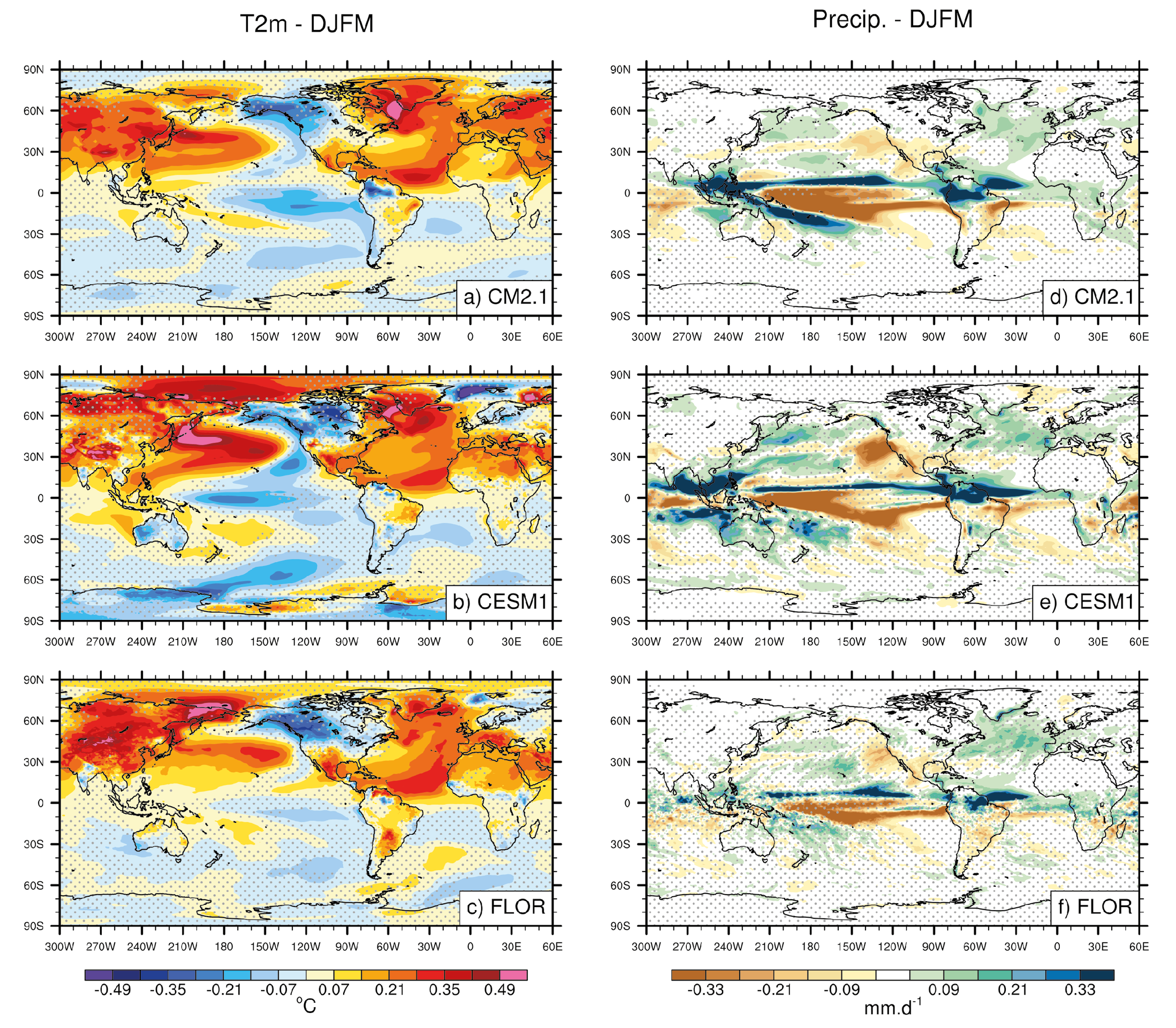
Figure 2: Differences between the 10-year average of the Full_AMV+ and the Full_AMV- ensemble simulations for December to March (DJFM) of (a, b, c) 2-meter air temperature and (d, e, f) precipitation. Results are shown from top to bottom for CM2.1, CESM1, and FLOR. Stippling indicates regions that are below the 95% confidence level of statistical significance according to a two-sided t-test. Note that the contours intervals of T2 in a, b, and c have been multiplied by 1.75 compared to Figure 1b. |
During DJFM, restoring the three models to the observed AMV yields, as expected, a North Atlantic warming (Fig. 2a-c). The temperature pattern of the simulated anomalies shows some differences with the observed one of Fig. 1b. Specifically, the relative strength of the SPG anomalies compared to the tropical anomalies is much less than the observed one. This comes from our choice to keep a time and space invariant restoring timescale for the SST. By so doing, the extratropical North Atlantic SSTs are weakened due to the SPG deep mixed layers, which dilutes the imposed SST anomaly over a deeper oceanic column.
Regardless of this weakness, we find that outside of the North Atlantic, the three models simulate remarkably similar global teleconnections. We note a slight warming of the Indian Ocean and a negative phase of the IPO over the Pacific. The latter has negative SST anomalies in the Tropical Pacific that extend toward the higher latitudes in both Hemispheres along the eastern ocean boundary, in a horseshoe-like pattern, surrounding positive SST anomalies in the West. The three models show a warming of ~0.3°C over Mexico and the Eastern part of US, a warming over East Brazil as well as over South Asia and the Mediterranean area. The models also agree on the simulated warming over Siberia and on the cooling of the northwestern part of North America. In response to AMV+ forcing, CESM1 simulates a significant warming of the Arctic that is only found over the northeastern rim of Siberia in CM2.1 and FLOR. The models also disagree on the temperature response over Northern Europe: CM2.1 simulates a warming there whereas CESM1 and FLOR tend to simulate a cooling.
We find that AMV leads to significant changes in the atmospheric winter circulation as illustrated by precipitation and geopotential height at 500 hPa (Z500) anomalies (Figs. 2d-f and Fig. 3b)2. There is a northward shift and a reinforcement of the Intertropical Convergence Zone all over the tropical belt as well as a southwestward shift of the South Pacific Convergence Zone. The precipitation response over the Tropical Pacific is coherent with a La Niña-like temperature pattern seen in Figs. 2a-b. We further analyzed the amplitude of the ENSO response3 and found that in all models the occurrence of La Niña events roughly doubles between the Full_AMV- and the Full_AMV+ experiments.
 |
|
Figure 3: Difference between the 10-year average of the positive and the negative phases of (a, b) Full_AMV, (c, d) Trop_AMV, (e, f) SPG_AMV for CESM1 in DJFM. (left) 2-meter air temperature (T2m) and (right) geopotential height at 500 hPa (Z500, color) and streamfunction of the wind at 200 hPa (SF200, contours at intervals of 0.8x10⁶ m2 s-1). Stippling indicates regions that are below the 95% confidence level of statistical significance. Figure adapted from Ruprich-Robert et al. (2017). ©American Meteorological Society. Used with permission. |
Over the extratropical North Pacific, the AMV leads to a weakening of the Aleutian Low (Fig. 3b) associated with an east-west dipole in the precipitation anomalies over the North Pacific and decrease of precipitation over the west coast of US and Mexico (Figs. 2d-f). The Z500 anomalies are reminiscent of the negative phase of the Pacific North America pattern (PNA) (Barnston and Livezey, 1987), with positive Z500 anomalies centered over the Aleutian Low and Mexico and negative anomalies over Canada and south of Hawaii. The latter center of action is more visible when looking at streamfunction anomalies at 200hPa (hereafter SF200; Fig. 3b).
The North Pacific SST response is also consistent with the Aleutian Low weakening as discussed by Zhang and Delworth (2015). In their study, they linked a northward shift of the westerlies to a northward shift of the oceanic gyre circulation through a Sverdrup balance and to the propagation of oceanic Rossby waves from the central Pacific to the western coast, explaining the warmer SST off Japan. Over the northeastern side of the North Pacific, the SST cooling is driven by an anomalous advection of cool air from the Arctic. Furthermore, this whole North Pacific response is reminiscent of that documented in the water hosing experiments of Zhang and Delworth (2005), Dong and Sutton (2007) and Okumura et al. (2009), although the impacts are weaker in our experiments as expected from the weaker imposed forcing.
While the North Pacific response is significant and robust among the three models, the North Atlantic – Europe (NAE) response is notably weaker. All models simulate an increase of precipitation over Southern Europe, but these anomalies are only significant in CESM1. In CESM1 and FLOR, these precipitation anomalies are associated with a weak anomalous north-south Z500 dipole that projects on the NAO in its negative phase (hereafter NAO-). The geopotential anomalies in CM2.1 do not project strongly onto the NAO, even though positive anomalies are present over Iceland. For CM2.1 this diagnostic suggests that the NAE atmospheric response might project onto a mix of both an NAO- and a negative phase of the East Atlantic Pattern4(not shown). We further quantified the signal-to-noise ratio of the climate response to AMV and, for all models we found that the NAE atmospheric response accounts for less than 10% of the decadal variance. The discrepancy between the models and the weak atmospheric response over the NAE region suggest that the AMV does not strongly impact the atmosphere over there. We acknowledge however that our experimental protocol may lead to an underestimation of the extratropical AMV forcing and hence potentially to an underestimation of the atmospheric response over the NAE region. Indeed, as discussed above, our choice to keep a time and spatially-invariant restoring timescale does not allow to strongly constrain the SST over a region with deep oceanic mixed layer such as the SPG.
b) Tropical vs Extratropical SST contribution to the AMV climate impacts
We investigated the respective contribution of the tropical and extratropical parts of the AMV to the climate impacts described in the previous section by performing two additional sets of experiments in which only the subpolar (SPG_AMV) or the tropical (Trop_AMV) parts of the AMV pattern were imposed. Only the results from the CESM1 experiments are shown here, but these experiments were also performed with CM2.1 and we discuss the results from both models. We find that the Pacific IPO-like and PNA-like responses are primarily driven by the tropical part of the AMV (Figs. 3c,d). This result corroborates the studies of Kucharski et al. (2015) and McGregor et al. (2014) who suggested that the tropical Pacific cooling observed during the last decades was forced by the tropical Atlantic warming through a modification of the Walker Circulation. In line with Sutton and Hodson (2005), we find that the AMV impacts over the Americas are mainly explained by the tropical part of the AMV but that they are reinforced by the subpolar part of the phenomenon (Figs. 3a,c,e).
The models show marginal impacts over North Africa and Europe in terms of T2m anomalies in response to the tropical AMV anomalies only, whereas a warming of North Africa and a cooling of Europe is simulated in response to the SPG anomalies. This cooling is consistent with the Z500 dipole anomaly seen over the NAE region, which tends to decrease the atmospheric flow from the relatively warm ocean to the relatively cool European continent in winter. Further, the Z500 dipole response in the SPG_AMV experiment is shifted eastward compared with the NAO response seen in the Full_AMV experiment (Fig. 3b). This suggests that the subpolar part of the AMV is the primarily driver of the NAE atmospheric response but that both the tropical and the extratropical parts of the AMV contribute to the overall NAE atmospheric response.
The SPG_AMV experiment generates a strikingly larger global atmospheric response in CESM1 than in CM2.1. For the former, the subpolar gyre part of the AMV leads to impacts in T2m and Z500 over the North Pacific region that are weaker but similar in pattern to those driven by the tropical part of the AMV. This is consistent with the weak but significant warming simulated in the tropical North Atlantic in the CESM1 SPG_AMV experiment. This also suggests that part of the tropical signature of the AMV is forced by the subpolar part of the AMV as suggested by Dunstone et al. (2011) and Smirnov and Vimont (2012) but that this mechanism is model-dependent.
Summary and discussion
We investigated the climate impacts associated with the internal component of the observed Atlantic Multidecadal Variability (AMV) using the GFDL-CM2.1, the NCAR-CESM1, and the GFDL-FLOR coupled models, by restoring their North Atlantic SSTs to the observed anomalies. This coupled approach allowed us to determine the full climate response to the imposed North Atlantic anomalies.
Over the North Atlantic European (NAE) region, we show that, despite the large-scale warming of the Northern Hemisphere continents simulated in all models during the boreal winter (DJFM), the models disagree on the Northern Europe temperature response. They disagree also on the NAE atmospheric circulation response, which projects on the negative phase of the North Atlantic Oscillation (NAO) for CESM1 and FLOR. The disagreement between the models and the weak signal-to-noise ratio of the NAE atmospheric response reveal strong uncertainties on the role played by the AMV in the decadal variations of the NAO observed during the last century. They also suggest the need to repeat such coordinated experiments with other models.
For the three models, we find that the AMV warming drives a change in the Walker Circulation that drives precipitation anomalies over the whole tropical belt. The AMV warming leads also to reduced rainfall over the western part of the US and Mexico and to a weak increase of rainfall over Europe. The Walker Circulation response is associated with broad Pacific anomalies that project onto the Interdecadal Pacific Oscillation (IPO) in its negative phase. In the three models the northern part of the IPO-like SST response is tightly linked to a negative phase of the Pacific North American teleconnection pattern (PNA). We find that both the IPO and PNA-like responses are mainly driven by the Tropical part of the AMV.
Our results stress the importance played by the North Atlantic Ocean variability associated with the AMV in driving decadal changes on a global scale, especially in the Pacific. They also indicate that the AMV has played an important role in global climate variability observed during the last century. In the present study, we specifically focus on the climate impacts associated with an estimate of the internal component of the observed AMV, which has been shown as predictable to some extent on multi-year to decadal timescale (e.g., Robson et al., 2012; Yeager et al., 2012; Msadek et al., 2014). Our results are therefore encouraging for the prospect of getting skillful decadal predictions over regions outside of the North Atlantic through the impacts of AMV. The teleconnections we highlight between the Atlantic and the Pacific are also consistent with the studies of Chikamoto et al. (2012, 2015), who showed that phase shifts of the IPO as those observed in the late 1990’s might be predicted few years in advance if the sign and amplitude of the AMV are predicted.
The general impacts and mechanisms described in the present study are based on three climate models that show quite similar results despite their different atmospheric resolution. This gives confidence in the robustness of our conclusions regarding AMV impacts. However, conducting such experiments within a multimodel framework, using other coupled climate models, will be highly beneficial to strengthen our conclusions. This will be done as part of the CMIP6 Decadal Climate Prediction Project (DCPP), which calls for coordinated experiments following a protocol similar to the one proposed in this study (Boer et al., 2016).
acknowledgements
The analysis and plots of this paper were performed with the NCAR Command Language (version 6.2.0, 2014), Boulder, Colorado (UCAR/NCAR/CISL/VETS, https://doi.org/10.5065/D6WD3XH5). NCAR is sponsored by the National Science Foundation (NSF). The CESM is supported by the NSF and the US Department of Energy. This work is supported by the NSF under the Collaborative Research EaSM2 grant OCE-1243015 to NCAR and by the NOAA Climate Program Office under the Climate Variability and Predictability Program grant NA13OAR4310138 to NCAR and GFDL.
affiliations
1Atmosphere and Ocean Sciences, Princeton University, and NOAA/GFDL, Princeton, New Jersey
2CNRS-CERFACS, Toulouse, France
Footnotes
1Defined as the December to March seasonal mean.
2In view of concision, only Z500 response from CESM1 is shown here, but we specify in the following when this response is different among the models.
3To do so, we defined an ENSO index based on the first EOF of the upper 200 m oceanic heat content computed over the tropical Pacific (30°S-30°N).
4This mode is defined in observations as the second mode of variability of the atmosphere over the NAE region (e.g., Barnston and Livezey 1987).
references
Castruccio, F., Y. Ruprich-Robert, S. Yeager, G. Danabasoglu, R. Msadek, T. Deloworth, 2017: Modulation of Arctic Sea Ice Loss by Atmospheric Teleconnections from Atlantic Multi-decadal Variability. Geophys. Res. Lett., in revision.
Clara Deser, Adam Phillips
Introduction
Due to their thermal and mechanical inertia, the oceans play a key role in decadal-scale climate variability (DCV) and provide a potential source of initial-value predictability for low-frequency climate fluctuations. Characterizing oceanic DCV is challenging, however, due to the limited duration of the observational record combined with the sparse and irregular data coverage. These constraints also hinder assessments of the robustness of the patterns and timescales of DCV, and understanding of the governing mechanisms. In this brief note, we provide an overview of the main phenomena of DCV in the historical sea surface temperature (SST) data record, discuss proposed interpretations and causal mechanisms, and highlight outstanding research questions.
SST data coverage
Our focus on SST is motivated by both practical and physical considerations. On the practical side, the longest ocean temperature records are measured near the surface from ships-of-opportunity, starting with bucket samples in the 19th and early 20th centuries followed by engine-intake measurements (e.g., Woodruff et al., 2008). On the physical side, SSTs are the main agent of communication between the atmosphere and the ocean, and thus represent a key quantity for probing DCV (for a discussion of the upper-ocean mixed layer heat budget, c.f. Deser et al., 2010).
 |
|
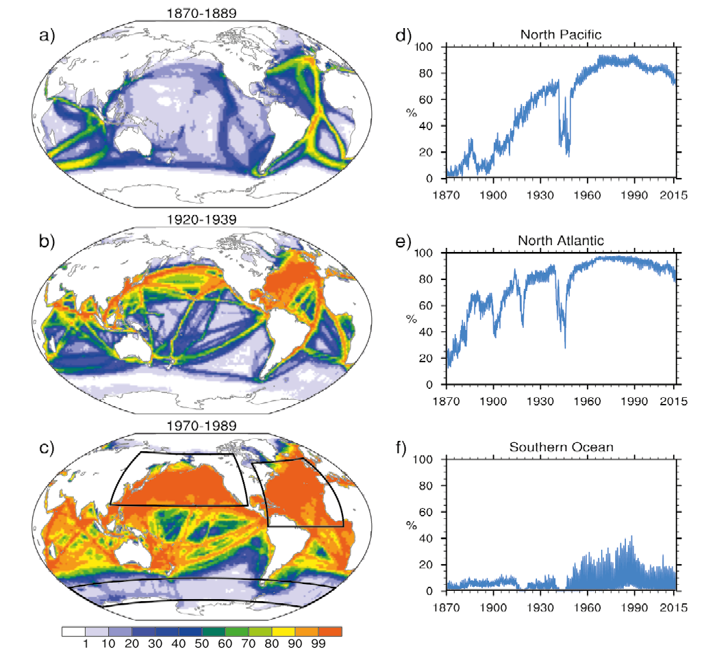
Figure 1: Distribution of sea surface temperature observations from the International Comprehensive Ocean Atmosphere Data Set. Maps show the percentage of months with at least one measurement in a 2 degree latitude by 2 degree longitude grid box during (a) 1870-1899, (b) 1920-1939, and (c) 1970-1989. Timeseries (1870-2015) show the percentage of grid boxes that have at least one observation per month within the regions outlined in Fig. 1c. (d) North Pacific (20°-70°N, 110°E-100°W), (e) North Atlantic (0°-60°N, 80°W-0°W), and (f) Southern Ocean (50°-70°S, 0°W-360°E). |
Fig. 1 (left column) shows maps of SST data coverage based on the International Comprehensive Ocean Atmosphere Data Set (ICOADS) (Woodruff et al., 2008) during three representative 20-year periods spanning the late 19th and 20th centuries: 1870-1899, 1920-1939, and 1970-1989. These maps show the percentage of months with at least one measurement in a 2° latitude by 2° longitude grid box in the 20-year period indicated. We note that the instrumental coverage falls off rapidly before 1870, and that satellites provide nearly global coverage starting in the 1980s (see Woodruff et al., 2008 and Deser et al., 2010). The discrete outlines of commercial shipping routes and their changes over time are readily apparent, especially in the earlier time periods (Fig. 1). Broadly speaking, the North Atlantic, western South Atlantic, and northern Indian Ocean contain the highest density of observations, with reasonable coverage back to approximately 1870. Data coverage in the North Pacific is limited before about 1920, in the Tropics before about 1960, and in the Southern Ocean before the advent of satellite remote sensing (Fig. 1). The uneven and changing spatial coverage of SST measurements from historical ship-based archives must be taken into account in any analysis of DCV. Further information on the spatio-temporal coverage of other SST data sets is available at climatedataguide.ucar.edu.
The main phenomena of DCV
In our view, there is no unique “best” approach to defining the main phenomena of DCV. Here, we adopt a basin-specific perspective, which has the advantage that any inter-basin linkages (including those lagged in time) are not built-in to the analysis protocol. Similarly, we analyze monthly data (lightly smoothed with a 3-point running mean) so as to avoid artificially building in any low-frequency behavior. In this regard, it is important to bear in mind the null hypothesis that any low-pass filtered time series will exhibit DCV, but it need not be physically meaningful (i.e., it may not be distinguishable from a random process).
We use the NOAA Extended Reconstruction Sea Surface Temperature, version 3b (ERSSTv3b) dataset, which employs a statistical procedure on the ICOADS data to fill in missing grid boxes (Smith et al., 2008); other data sets yield similar results (not shown). Following previous studies, we subtract the global mean SST anomaly (SSTA) from the SSTA at each grid box for each month and year (hereafter, we use the nomenclature SSTA* to denote this residual from the global mean) unless noted otherwise. This procedure is intended to remove any secular global trends that may be associated with changes in external radiative forcing such as those due to human-induced increases in greenhouse gas concentrations and sulfate aerosols accompanying fossil fuel burning. We shall return to the issue of how well this procedure achieves its intended purpose in Section 5.
We define the main phenomena of DCV for each basin separately as follows. North Pacific (NPAC): leading principal component (PC) time series of monthly SSTA* over the domain (20°-70°N, 110°E-100°W) following Mantua et al. (1997). North Atlantic (NATL): time series of SSTA* averaged over the domain (0°-60°N, 80°W-0°W) following Trenberth and Shea (2006). Southern Ocean (SO): time series of SSTA (not SSTA*) averaged over the domain (50°-70°S, 0°W-360°E) following Fan et al. (2014). We have inverted the SO time series to facilitate comparison with NPAC and NATL. These regions are outlined in Fig. 1c. To obtain the global-scale patterns associated with each time series, we regress SSTA* (SSTA for the case of the SO) at each grid box on the standardized index time series.
Before showing the spatial patterns of DCV, we return to the issue of data coverage. The right-hand panels of Fig. 1 show time series of data coverage in each region defined above, represented as the percentage of grid boxes that have at least one observation in each month. Consistent with the data coverage maps, the NPAC region shows >50% of grid boxes with at least one observation starting around 1920 except during the 1940s (Fig. 1d). The NATL region shows >50% of grid boxes present since about 1885 except for the World Wars and around 1900 (Fig. 1e). Finally, coverage in the SO region is always <40%, and <10% before 1950 (Fig. 1f). A large seasonal cycle is evident in the SO region, with peak coverage during summer (Fan et al., 2014). In view of these results, we choose to show the NPAC and NATL time series starting in 1890 (mindful of the reduced coverage in NPAC before 1920), and the SO record starting in 1950. However, the global regression maps are all based on the period since 1950 to accommodate the lack of data over the Southern Ocean (and to a lesser extent, the Tropical Pacific) before that time.
 |
|
Figure 2: Spatial and temporal characteristics of sea surface temperature anomaly (SSTA) variability in selected ocean basins. (Left column) Global SSTA* regression maps (degrees C) based on the (a) leading principal component of North Pacific SSTA*, (b) North Atlantic SSTA*, and (c) inverted Southern Ocean SSTA. All indices were standardized prior to computing the regression maps. Index regions are outlined by black boxes. (Right column) Standardized 3-month running mean time series (1880-2015) of the (a) leading principal component of North Pacific SSTA*, (b) North Atlantic SSTA*, and (c) inverted Southern Ocean SSTA. Asterisk indicates that the global mean SSTA was removed prior to computing the time series and regression maps. |
The three SSTA* patterns show a great deal of similarity in their global structures, despite that they are based on different index regions. For example, NPAC shows a pan-Indo/Pacific pattern with symmetry about the equator, reminiscent of the low-frequency “tail” of ENSO (also termed the “Pacific Decadal Oscillation PDO or “Inter-Decadal Pacific Oscillation IPO) (Zhang et al., 1997; Power et al., 1999; Vimont, 2005; Newman et al., 2016). It also features linkages to the Atlantic in the form of alternating polarities with latitude, with positive values over the northern North Atlantic, and negative values over the Pacific sector of the Southern Ocean (Fig. 2a). NATL exhibits an out-of-phase relationship between SSTA* in the North and South Atlantic, distinct from that based on NPAC (Fig. 2b). However, it shares the same SSTA* polarity over the northern NATL and the same PDO-like structure, albeit with weaker magnitude, as that based on NPAC, and it shows negative values throughout the Southern Ocean (Fig. 2b).
Finally, the pattern based on the (inverted) SO index is very similar to that based on NATL, except for the sign over the northern tropical Atlantic (Fig. 2c).
The NPAC, NATL and SO index time series are remarkably similar during their period of overlap (1950-2015), with pronounced decadal-scale variability evident even in 3-month running mean data (Figs. 2d-f). In particular, each record swings from positive to negative and back to positive during 1950-2015, with a suggestion that NATL leads NPAC and SO by 10-20 years. Before 1950, NPAC shows less prominent decadal-scale variability and a weaker relationship with NATL than after 1950. We refrain from quantifying these statements due to the low number of degrees of freedom associated with such short records of DCV.
Causes of DCV
The substantial degree of commonality in the global-scale patterns associated with Pacific, Atlantic and Southern Ocean DCV, combined with the fact that they are based on short records and sparse sampling, make it challenging to identify these phenomena robustly in terms of spatial and temporal character. These constraints also make it difficult to assess whether they arise from distinctive dynamical processes operating on decadal time scales and/or whether they are best viewed as manifestations of a “random walk” process or processes (see also Newman et al., 2016). The concept of global-scale SSTA “hyper-modes” (Dommenget and Latif, 2008; Dommenget, 2010; Clement et al., 2011) has been advanced to account for the similarity of global-scale SSTA patterns regardless of how they originate. This concept relies on the notion that the lower the frequency, the more global the pattern, due to the interplay between SSTA and the large-scale atmospheric circulation.
These issues highlight the need for a combined approach based on observations, paleo-climate records and modeling to delineate robust phenomena of DCV and to understand their causes. Indeed, modeling studies based on thousands of years of simulation for robust statistics suggest that Atlantic DCV and its global-scale teleconnections may originate from the mutual interaction of the oceanic Atlantic Meridional Overturning Circulation (AMOC) and the large-scale atmospheric circulation in the form of the North Atlantic Oscillation (NAO) (Delworth et al., 2016; Delworth and Zeng, 2016; Ruprich-Robert et al., 2016), although the mechanisms continue to be under investigation. Similar conclusions arise for Southern Ocean DCV (Latif et al, 2013; Latif et al., 2015; Zhang et al., 2016). Finally, Pacific DCV may reflect a combination of stochastic processes, each with a different decorrelation time scale and regional emphasis arising from dynamical and thermodynamic air-sea interaction (Clement et al., 2011; Okumura, 2013; Newman et al., 2016).
Internal vs. externally-forced DCV
As mentioned above, DCV is traditionally identified as the residual from the global mean SSTA; the latter interpreted as the secular fingerprint of human-induced climate change. However, human-induced climate change is not spatially uniform (Xie et al., 2010) and thus the removal of the global-mean SSTA may fall short of its intended purpose. The validity of this approach can be tested with large initial-condition ensembles of historical simulations with comprehensive coupled climate models, such as 40-member Community Earth System Model Large Ensemble (CESM-LE) (Kay et al., 2015). The CESM-LE has been used to isolate externally-forced and internally-generated components of simulated NATL DCV, with implications for observed NATL DCV (Tandon and Kushner, 2015; Murphy et al., 2016). These studies indicate that a significant portion of NATL DCV since 1920 may be externally-forced, and that empirical methodologies used to separate these components in the single observational record may be inadequate. Further work is needed to evaluate the efficacy of empirical approaches for separating forced and internal components of DCV, not only in the NATL but in other ocean basins as well. These approaches include linear (or other forms of) detrending, removal of the global-mean, optimal fingerprinting (Ting et al., 2009; Ting et al., 2014), pattern scaling (Hoerling et al., 2011; Bichet et al., 2015), and Empirical Ensemble Mode Decomposition (Wu et al., 2011).
Concluding remarks
We have presented a brief overview of the main phenomena of DCV based on simple analyses of observed SST over the historical record using a basin-specific approach. Our results indicate that DCV is apparent even in unfiltered seasonal data, and that DCV in the North Atlantic, North Pacific and Southern Ocean share many characteristics including their global-scale patterns and chronologies, especially since 1950. Results are more ambiguous before that time. Given the shortness of the observational record relative to the time scales of interest, we believe that DCV is best viewed in terms of a case study approach rather than as a robust and stationary statistical characterization. Long (thousands of years) model control simulations provide an effective tool for assessing the robustness and global-scale linkages of DCV, provided the model has a credible representation of the relevant processes governing DCV. Finally, an outstanding research question is the extent to which DCV is externally-forced vs. internally-generated.
affiliation
National Center for Atmospheric Research, Boulder, USA
references
Yochanan Kushnir, Christophe Cassou, Scott St George
The study of Decadal Climate Variability and Predictability (DCVP) is the interdisciplinary scientific enterprise to characterize, understand, attribute, simulate, and predict the slow, multi-year variations of climate on global and regional scales. Particular interest in decadal climate variations and their role in the global surface climate change stems from the need to detect and attribute the uneven rise in global mean surface temperatures (GMST) since the beginning of the industrial period. The most recent expression of decadal variability in GMST has been the slowdown in warming between roughly 1998 and 2012. This period, often termed as the “hiatus”, triggered intensive debate in the public domain, even if global temperatures had exhibited long undulations before, including two cooling events in the late 19th to early 20th century and in the mid 20th century and two intervals of rapid warming, one from about 1910 to 1940 and the other between the early 1970s and 1998. While these departures from the expected warming due to the steady increase in greenhouse gas forcing have been attributed in part to natural (volcanic) and anthropogenic (industrial) aerosols, there is ample evidence that long-term internal interactions between climate system components – the ocean and the atmosphere, in particular – have also been involved.
Decadal and longer variations in sea surface temperatures (SSTs) have a rich and non-uniform spatial pattern related to variations in the distribution of precipitation and associated atmospheric convection in the tropics, to alterations in position and strength of the storm tracks at midlatitudes, to changes in sea-ice extent at polar latitudes in both hemispheres, etc. Changes in atmospheric circulation thus contributes to changes in regional climates worldwide and importantly over the continents, directly affecting humans and their environment. The most prominent example of the terrestrial response to decadal climate variability is the long-lasting decline of rainfall in the North African Sahel in the second half of the 20th century, which included the devastating famines of the 1970s & 1980s. These decadal-scale shifts have been attributed to slow variations in North Atlantic SSTs, which have also affected Atlantic tropical cyclone activity over the same time frames. Similarly, the multi-year pulses of North American droughts (e.g., the Great Plains “dust bowl” in the 1930s and the recent protracted dry period in the Southwest US), which impacted lives and livelihoods in the US and northern Mexico, have been attributed to the state of the tropical Pacific and tropical Atlantic Oceans. For the Mediterranean region, in South European countries along the northern rim and in the Maghreb and the Middle East, recurrent heat waves and prolonged dry spells since the mid 1960s, attributed to a combination of internal decadal variability and greenhouse gas forcing, have devastated regional agriculture productivity, lead to loss of life and, perhaps arguably, to widespread societal instability and in Syria to violent conflict and war.
In order to anticipate the impacts of climate change, it is important for society to know how the climate response to anthropogenic forcing and the climate impact of natural variability will mix together to affect the near-term future. The study of DCVP aims to provide science-based information to decision makers through research, observations, and decadal predictions. This goal remains challenging despite decades of research and of extensive progress in observing and modeling the climate system. Predicting the impact of internal decadal climate variability is complicated by our incomplete understanding of the nature of the underlying phenomena, in particular their physical origins and their interaction with external forcing. Existing obstacles in DCVP research thus test our ability to attribute past variations to the combined role of internal variability and external forcing, as well as to reliably predict the near-term climate on global and regional scales.
Progress in DCVP research can only be made through international, cross disciplinary collaborations between scientists. Because of the difficulties to observe and model the Earth’s climate at timescales of a decade or longer, this area of research is wholly dependent on emerging connections between those who perform, collect and analyze instrumental observations of the present, those who develop and analyze proxies of past climate, and with scientists who develop models and perform dedicated modeling experiments. To review ongoing research on DCVP and propose the road to future progress on the subject, the International WCRP CLIVAR Project and PAGES held an international workshop with representatives of these various disciplines in November of 2015, under the patronage of the International Centre for Theoretical Physics in Trieste Italy. This issue of Exchanges grew out from the presentations and discussions features in this workshop.
The articles in this issue of Exchanges were selected and reviewed by the members of the CLIVAR Working Group on DCVP and the PAGES 2k Network. These contributions are meant to provide brief reviews that address the progress made in understanding and resolving different key issues in DCVP. We greatly appreciate the voluntary efforts made by these authors to capture the exciting and rapidly growing literature on the subject in these brief summaries and hope that they will stimulate further research collaboration on the subject.
Claudio Latorre1,2, J.M. Wilmshurst3,4 and L. von Gunten5
From megafauna hunters in Patagonia to the fantastic civilizations in Chaco canyon, the Maya or settlers of remote oceanic islands, this issue aims to highlight how social decisions in the face of environmental change had long-lasting consequences for the evolution and development of prehistoric societies. Many regions of the world have undergone climate change since their first occupation by humans, and understanding how people who settled these places chose to confront or adapt (or failed to adapt) may play a vital role in sustainable planning of our modern societies.
From demographic collapse to social complexity, cultural evolution is an incredibly broad and complex topic at the forefront of much archaeological and anthropological research today. By affecting the availability of food and water to human populations, environmental drivers are a key factor for understanding this process. It is, however, an oversimplification to state that environmental drivers, such as climate change, are directly responsible for cultural change. Although there are many examples in the literature of large civilizations that suffered some degree of collapse, to attribute these social changes solely on shifting climate states (drought and the Maya is one particularly cited example) ignores other complex processes associated with how human societies make decisions regarding resource constraints.
 |
|
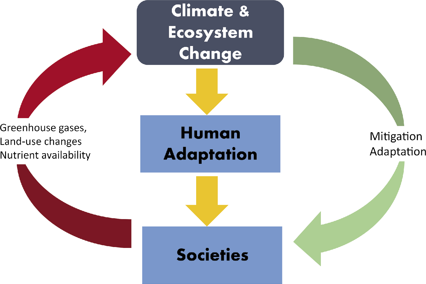
Figure 1: The relationship between humans and climate is complex and involves multiple feedback loops. As climate and ecosystems change over time, humans as organisms adapt to survive but as societies they can, in turn, influence the direction of future ecosystem change. This then feeds back into the decisions societies make to adapt to ongoing change as well as mitigation strategies. |
However, the effects of climate change on past (and indeed future) societies cannot be understated and there are often multiple feedbacks (Fig. 1). Case by case comparative studies can bring out commonalities across cultures, varying geographies and global climate shifts. Such is the spirit behind this issue of Past Global Changes Magazine. We have brought together a series of examples, from most of the major continents and several island groups, to try to understand the underlying processes of how climate and environmental change affected cultural evolution and social decisions. The contributions combine archaeological records with the vast amount of paleoecological and climate proxy information that is now available for many of these regions.
Some of the oldest interactions between humans and the environment discussed in this issue are from South America, the last continental landmass to be colonized by migrating humans at the end of the Pleistocene. One of the best examples for showcasing the complex nature of human-environment interactions is summed up by Maldonado et al. (p. 56), in which, despite inhabiting one of the driest deserts on earth, the early peopling of the Atacama involved a series of choices regarding their environment. Further south in Patagonia, Villavicencio (p. 58) shows how climate and humans clearly must have interacted through ecosystem change to explain the demise of the endemic megafauna at the southernmost tip of the continent.
The impact of extended and persistent drought reconstructed from paleorecords is a unifying theme for several of the contributions in this issue. Zerboni et al. (p. 60) show how the end of the African Humid period during the mid-Holocene brought about new forms of social complexity and societal resilience, and question if extreme oscillations in climate brought about the end of major regional civilizations. In contrast, Weiss (p. 62) shows that mega-droughts lasting several centuries at ca. 4 ka BP brought about synchronous collapse of the major civilizations that occupied the Middle East and Mesopotamia.
Much more contested, however, is the role of drought in bringing about major social change in the Americas. As shown by Beach et al. (p. 66), topography as much as climate may explain the diverse social responses to the onset of drought conditions towards the end of the “Classic” Maya period. Such a complex relationship may also explain the abandonment of the “great houses” of Chaco Canyon in New Mexico, USA, some 900 years ago during the Medieval Climate Anomaly. Betancourt and Guiterman (p. 64) provide us with an up-to-date review of the major aspects of this debate and stress that resource exhaustion and distribution problems may have played a pivotal role.
Oceanic islands were among the last areas to be occupied by prehistoric humans, who spread over the planet during the late Holocene. Rull et al. (p. 70) show that much still needs to be done to understand the waxing and waning of the Rapa Nui on Easter Island. Fernández-Palacios et al. (p. 68) highlight how recent human settlement over the last few thousand years has transformed the diverse Macaronesian island environments, but how they interacted with climates over this time is an area needing further research effort. Finally, Holz et al (p. 72) return to southern Patagonia to bring up the issue of how fire can be a critical parameter for assessing the impact of human-environment-climate interactions, especially in regions where naturally caused fires were infrequent.
affiliations
1Departmento de Ecología & Centro UC del Desierto de Atacama, Pontificia Universidad Católica de Chile, Santiago, Chile
2Institute of Ecology & Biodiversity, Santiago, Chile
3Longterm Ecology Lab, Landcare Research, Lincoln, New Zealand
4School of Environment, The University of Auckland, New Zealand
5PAGES International Project Office, Bern, Switzerland
contact
Claudio Latorre: clatorre bio.puc.cl
Antonio Maldonado1, C.M. Santoro2 and Escallonia members3
Prehistoric human groups in the Atacama Desert developed socio-cultural complexities despite living in the world’s driest desert. Different technological adaptations were developed as part of their interactions with variable environments over the last 14,000 years.
 |
|
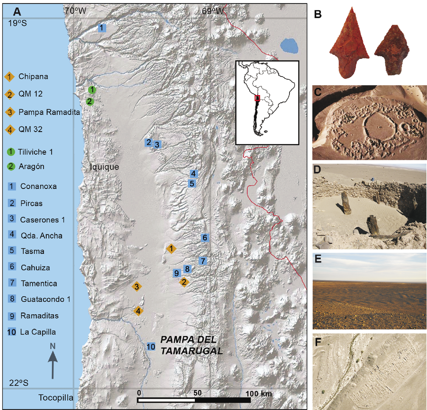
Figure 1: (A) Location of Early- (orange), Mid-Holocene (green) and Formative (blue) sites. (B) Late Pleistocene projectile points. (C, D, F) Formative villages. (E) Cropfields in Guatacondo. Red line shows today's border between Chile and Bolivia. |
Human history can be understood as the constant mutual interaction between variable environments and social systems. It is the basis for many archaeological and socio-natural science studies worldwide and is particularly prominent in the Atacama Desert in northern Chile. Using an eco-anthropological perspective, we focus on identifying and explaining social continuities and discontinuities that occurred during key cycles of water availability since the first humans arrived, ca. 14 ka ago, at the Pampa del Tamarugal (PdT), in the hyperarid core of the Atacama Desert (Fig. 1). The major trends of long-term history of human-environment interactions show that people developed different ways of living, to endure the desert even during the driest climatic periods instead of completely abandoning it or, even worse, suffering cultural collapse.
The first peoples in Pampa del Tamarugal and Tarapacá region (14-10 ka BP)
Ecosystems and human societies in the Atacama Desert have been constrained mainly by the lack of water. The first human occupation occurred at the end of the Pleistocene, during relatively moist periods (at 17.5-14 and 13-10 ka BP; Quade et al. 2008). In the PdT, these humid periods increased perennial stream discharge and groundwater tables, expanding riparian and wetland ecosystems into what is now the hyperarid core of the desert (Gayo et al. 2012; Fig. 2). During those humid periods, the desert became an attractive habitat for hunter-gatherers, plenty of camelids (i.e. guanacos and vicuñas), rodents and birds. The archaeological evidence shows human occupations next to paleowetlands surrounded by trees (i.e. Prosopis species parkland), the dry trunks of which are still preserved and visible on the surface of the desert (Santoro et al. in press; Fig. 1). Diverse contemporaneous open camps, like QM12 (Fig. 1 and 2), show complex hunting-gathering systems successfully adjusted to the ecosystems in the PdT, coupled with long-distance human interaction from the Pacific coast and the high Andes.
Environmental stress and socio-environmental discontinuity (10-3 ka BP)
 |
|
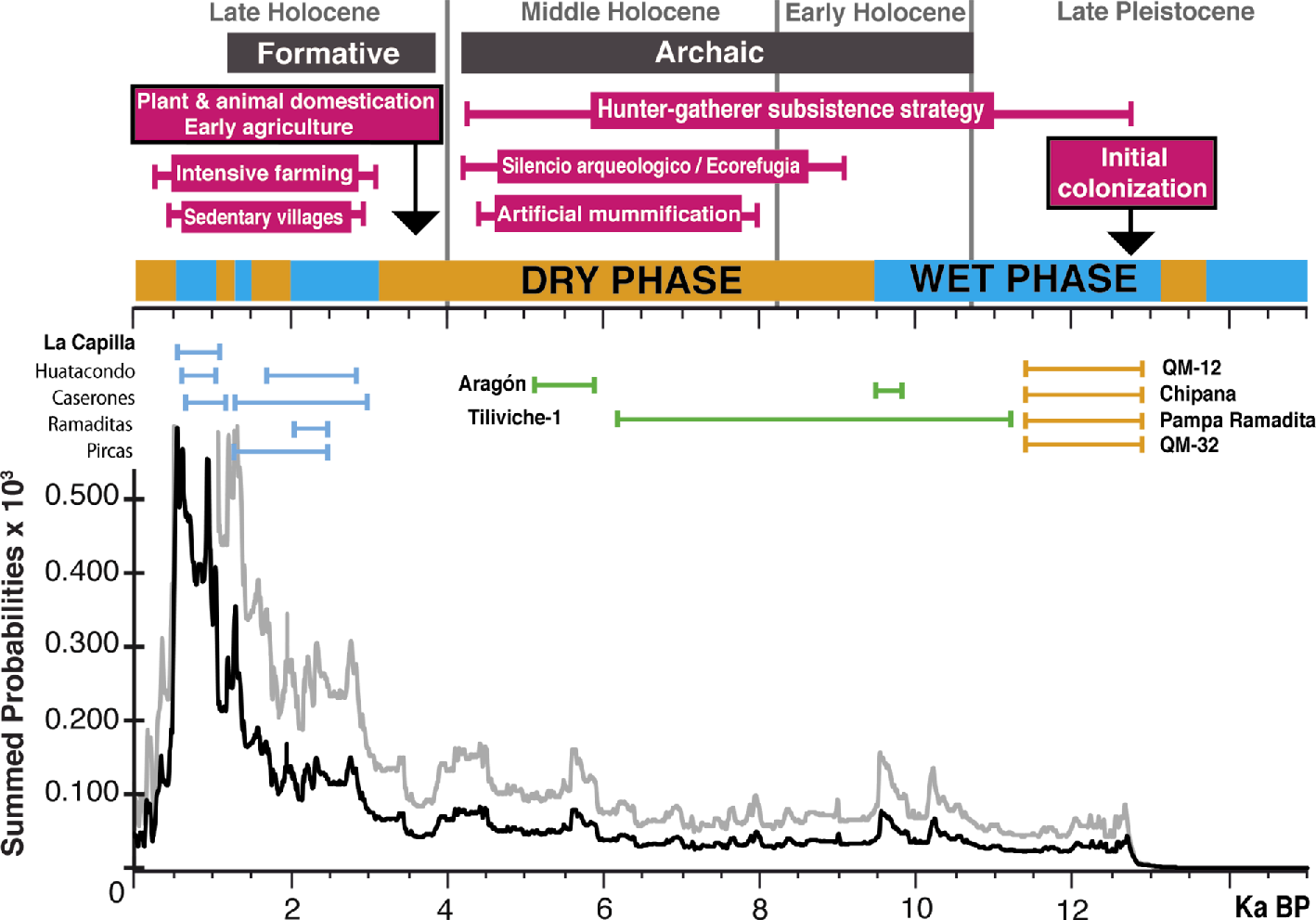
Figure 2: Paleoenvironmental and archaeological synthesis of the PdT since the Late Pleistocene showing human occupation modes, dry/wet phases, main archaeological sites (Fig. 1) occupation timing and occupation density (black line) measured through the summed probability 14C ages from archaeological sites in the PdT. The grey line is a 2x exaggeration of the black line. Modified from Santoro et al. (2016). |
The beginning of the Holocene (ca. 10 ka BP) seems to have triggered drastic transformations in settlement patterns and cultural behavior that lasted for several millennia due to the establishment of fluctuating arid conditions in the southern Atacama Desert (Núñez et al. 2013; Fig. 2). Archaeological data show a phenomenon of socio-environmental discontinuity that has been conceptualized as the “silencio arqueológico” (archaeological silence; Núñez et al. 2013).
Particularly in the PdT, the onset of hyperarid conditions triggered ecological stress characterized by the dramatic reduction of productivity in the ecosystem. Accordingly, people possibly migrated toward more productive areas such as the coast, where sequences of continuous occupation began approximately 9 ka BP, with complex ideological innovations, including artificial mummification (Marquet et al. 2012) and the development of a specialized technology focused on the exploitation of marine resources. More abundant settlements and the development of new technologies occurred along the coast since 7 ka BP (Castro et al. in press). The Altiplano, located eastwards of the PdT, was also productive as it may have been less vulnerable to climate change and maintained sustained environments (Ledru et al. 2013) and key locations for hunter-gatherers during the arid Mid-Holocene (Pintar 2014). Archaeological data show intensification in occupation after 10 ka BP. Other groups might have settled around local sources of permanent water within the PdT, or within narrow ravines such as Sapiga and Tiliviche canyons, whose archaeological sites (Aragón and Tiliviche 1; Fig. 1) point out that local ecosystems were complemented with protein from coastal resources (Santoro et al. in press).
Evidence from the central Atacama also shows, however, that populations rebounded after 6 ka BP, meaning that the Mid-Holocene may not have been as dry as thought (Gayo et al. 2015; see Fig. 2).
The return to the Pampa del Tamarugal (3-1 ka BP)
In the late-Holocene in the PdT, between 2.5-0.7 ka BP, arid conditions gradually gave way to wetter climates, peaking between 2-1 ka BP (Maldonado and Uribe 2015; Fig. 2). The wet phase is partly coeval with the cultural Formative period (2.5-1.5 ka BP), which is characterized by an intensification of social complexity and diversification of communities. Large, dispersed or concentrated villages with monumental public spaces were founded. A wide range of innovative technologies (i.e. ceramic, textile and metal production) and landscape arrangements were added to the traditional hunting-gathering systems. This involved sophisticated technologies for managing surface water including water dams, irrigation canals and farmland. These innovations generated a concentration of population and social power (Urbina et al. 2012; see Fig. 1a), coupled with an increase in population size (Gayo et al. 2015; see Fig. 2).
Internodal areas (1.0-0.5 ka BP) and capitalism (0.5 ka BP – present day)
Aridity, which increased from 1.0 to 0.7 ka BP and lasted until recent times, has been associated with sociopolitical turmoil and inequities (Uribe 2006). This resulted in massive population migrations to highland areas and the establishment of new and numerous settlements on the western slope of the Andes, since water resources in these areas were much more abundant and predictable (Maldonado and Uribe 2015; see Fig. 2). Consequently, new systems of agriculture (terraces and irrigation canals), strategic and defensive urban arrangements, and land management were developed. Increasingly circumscribed territories were managed by societies of “segmented” organizations (social groups independently organized). Thus, the PdT was transformed into an inter-nodal territory crossed by trains of llama caravans that connected the highlands with the coast.
During the Inca State regime (0.5-0.4 ka BP), the scale and organization of mining exploitation of copper and silver ore became important; thus, previous socio-economic systems were restructured for metal production (Zori and Tropper 2010). Traditional activities (i.e. agriculture, herding and foraging) gradually increased or intensified. The Spanish conquest (0.4-0.2 ka BP) brought new political, technological, demographic, and land-use conditions which changed the socio-environmental systems of the Atacama Desert. A proto-capitalist regime was introduced, focusing on the exploitation of raw materials, particularly minerals, which have dramatically stressed the human-environment relationships until today.
Discussion
The scale, intensity and continuity of human adaptive strategies in relation to fluctuating ecosystem resources have been diverse and variable throughout the last 14 ka BP in the Atacama Desert. Major humid or dry periods impacted the socio-environmental systems of hunter-gatherers, as well as the human occupation and the use of resources. Around 3 ka BP, a new, though less-intense, pulse of increased rainfall in the highlands reactivated ground- and surface-water flow in the hyperarid core of the Atacama. This boosted the development of complex water management technologies, and new social and ideological structures featured by the proliferation of people in the PdT. These innovations were also triggered by internal socio-cultural factors, which were capitalized by some communities in the PdT (e.g. Caserones village). The end of the wet period during the late Holocene (1.0-0.7 ka BP) led communities from the highlands and the coast to enlarge and improve novel systems of land use and management in the PdT. A new socio-political order dominated by segmented societies developed and lasted until the Inca epoch. This scenario was the base of the colonial and republican historical processes which accelerated the exploitation of desert environment resources. Both the environmental fluctuations and the people decisions based on cultural and social interests should be considered to explain the full range of complex sociopolitical variability in the PdT throughout the prehistory in the Atacama Desert.
acknowledgements
CONICYT/PIA grant project ANILLO SOC1405.
affiliations
1Centro de Estudios Avanzados en Zonas Áridas, Universidad de La Serena, Chile
2Instituto Alta Investigación, Universidad de Tarapacá, Arica, Chile
3M. Uribe, M.E. de Porras, J. Capriles, E.M. Gayó, D. Valenzuela, D. Angelo, C. Latorre, P.A. Marquet, A. Domic, V. McRostie, V. Castro
contact
Antonio Maldonado: amaldonado@ceaza.c
references
Castro V et al. (in press) Chungara 48
Gayo EM et al. (2012) Earth Sci Rev 113: 120-140
Gayo EM et al. (2015) Quat Int 356: 4-14
Ledru MP et al. (2013) Holocene 23: 1545-1557
Marquet PA et al. (2012) PNAS 109: 14754-14760
Núñez L et al (2013) Quat Int 307: 5-13
Pintar E (2014) Chungara 46: 51-71
Quade J et al. (2008) Quat Res 69: 343-360
Santoro CM et al. (in press) J Anthropol Archaeol, doi: 10.1016/j.jaa.2016.08.006
Urbina S et al. (2012) Bolet Museo Chile Arte Precolombino 17: 31-60
Zori CM, Tropper P (2010) Bolet Museo Chile Precolombino 15: 65-87
Natalia A. Villavicencio
The chronology of megafaunal extinctions in southern Patagonia suggest that they are due to a combination of human impacts, and vegetation and climate changes. Most extinct megafauna coexisted with humans for a relatively long time, and died out at different times.
By the end of the Pleistocene, the world lost most of its large mammal species in what is known as the Late Quaternary extinction event (LQE; Martin and Klein 1984), the magnitude and timing of which differs among continents (Koch and Barnosky 2006). For more than five decades, the discussion about the possible causes of extinction has revolved around the human impacts caused by modern humans moving out of Africa, climate changes associated with the glacial-interglacial transition or combinations of both (Martin and Steadman 1999). South America was one of the most severely impacted continents, losing around 82% (53 genera) of all its large mammal species with average body mass exceeding 44 kg (Brook and Barnosky 2012). In South America, human arrival and late glacial climate changes occurred within a relatively short span of time, although marked regional differences are present in both the timing and direction of climate change. These regional differences provide opportunities to test possible synergistic effects of these changes in driving the LQE (Barnosky and Lindsey 2010).
The case of Southern Patagonia
 |
|
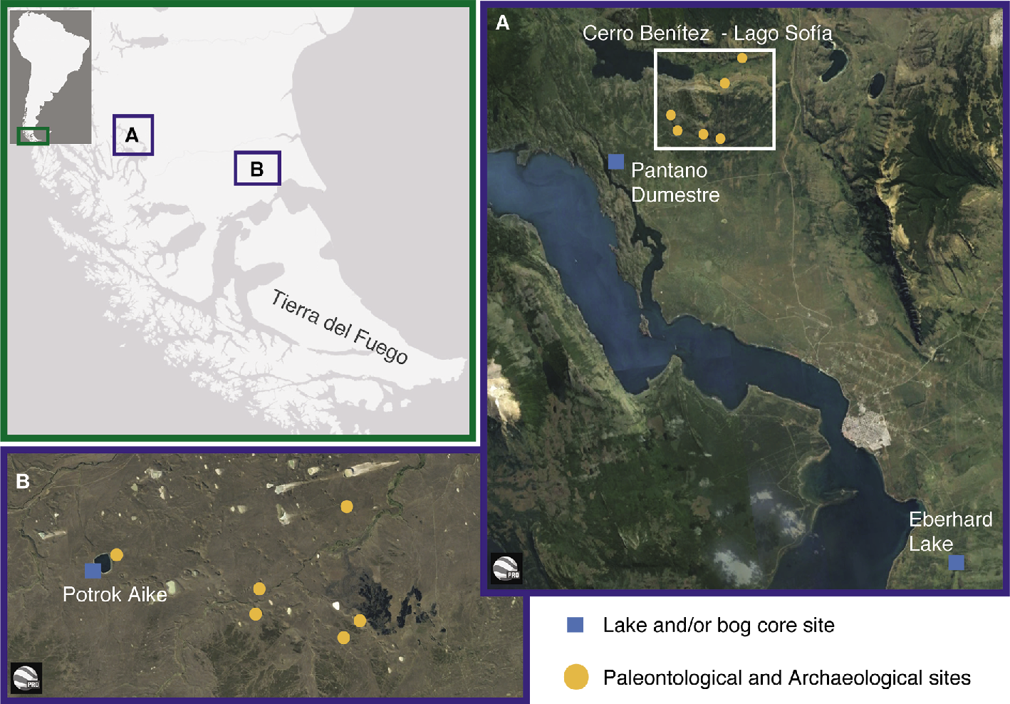
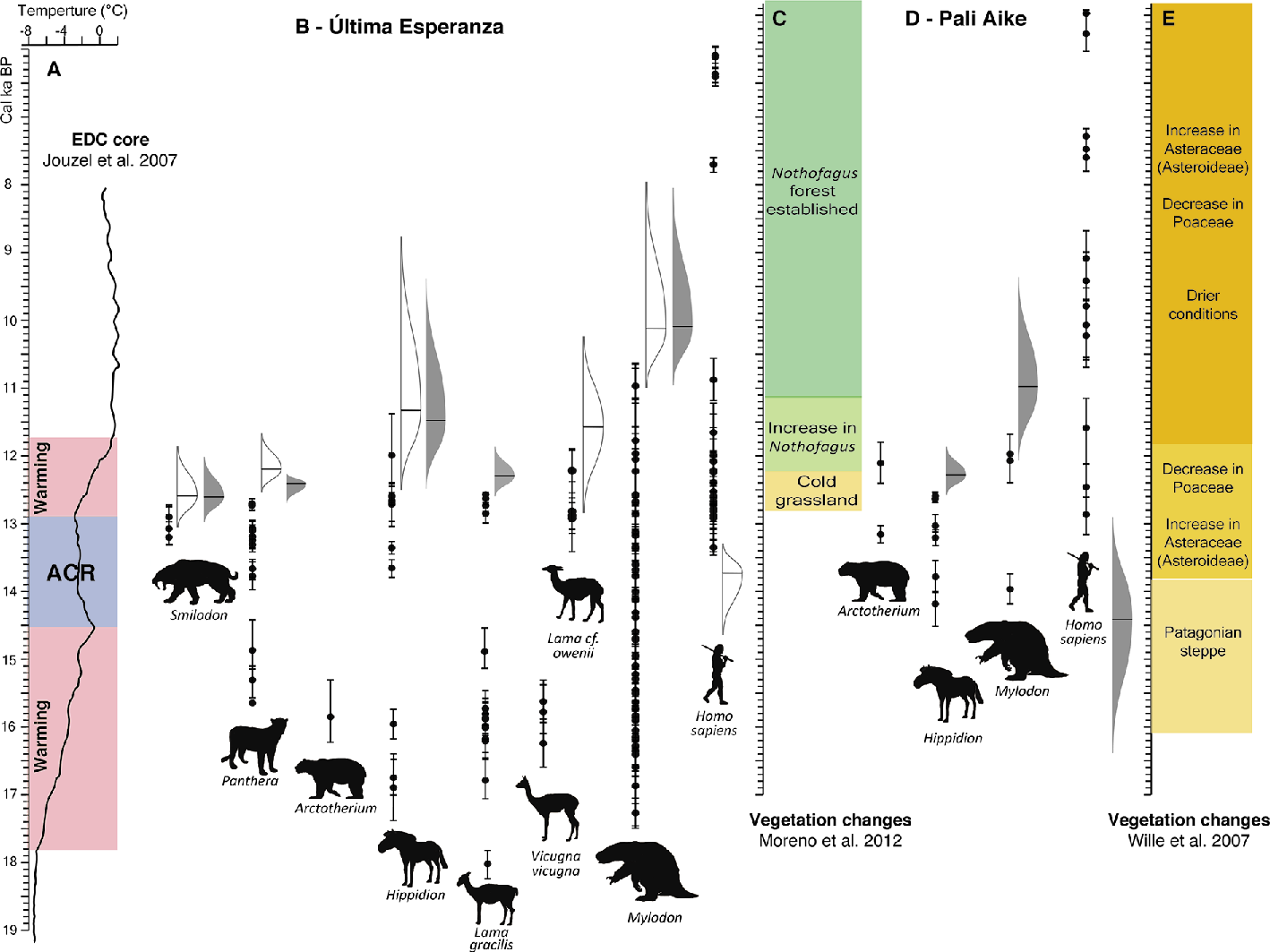
Figure 1: Map of southern Patagonia and location of study sites. (A) Última Esperanza, (B) Pali Aike. |
Several decades of research in caves and rock shelters in the area of Última Esperanza, Tierra del Fuego and Pali Aike (Fig. 1) have resulted in rich collections of extinct megafauna and evidence of the earliest human inhabitants in the area. Particularly, intense work in the Cerro Benítez and Lago Sofía area has produced dozens of radiocarbon dates on extinct fauna and helped establish one of the most complete chronologies of megafaunal extinction available from South America. Villavicencio et al. (2016) reviewed radiocarbon chronologies of megafaunal extinction and of human occupation from Última Esperanza, and the timing of major changes in climate and vegetation. Their main conclusions were (Fig. 2): First, mega-carnivores (Panthera and Smilodon) disappear slightly before the extinction of most of the herbivores, contrary to what is expected in a situation of trophic collapse. Second, Hippidion, Lama cf. owenii and mylodontids apparently coexisted with humans for hundreds of years (Hippidion and Lama cf. owenii) to millennia (mylodontids), ruling out a scenario of rapid overkill of these taxa by humans. Finally, Hippidion and Lama cf. owenii disappeared when cold grasslands were replaced by Nothofagus forest, followed by mylodontids disappearance, which occurred when the forests finally dominated the landscape.
Megafaunal extinctions in Última Esperanza
 |
|
Figure 2: (A) Temperature record from the EPICA Dome C ice core, Antarctica. Blue bar: Antarctic Cold Reversal, red bars: warming events (Jouzel et al. 2007); (B and D) Chronology of megafaunal extinctions and human arrival in Última Esperanza (modified from Villavicencio et al. 2016) and Pali Aike; (C and E) Vegetation change estimations for Última Esperanza (Moreno et al. 2012) and Pali Aike (Wille et al. 2007). Black circles: direct calibrated (Calib 7.04; Stuvier and Reimer 2014) radiocarbon dates on extinct megafauna and human evidence. The GRIWM best-estimates of extinction timing (or timing of human arrival) are indicated by the unshaded (Villavicencio et al. 2016) and shaded (this work) normal distributions, with the 95% confidence band depicted by the areas around the mean (black line: most probable time of extinction). |
Over 45 new radiocarbon dates on extinct megafauna in Última Esperanza were recently published (Metcalf et al. 2016; Martin et al. 2015), making an update of previous analyses possible by combining these new dates with the Villavicencio et al. (2016) dataset of 62 high-quality radiocarbon dates. In the combined dataset, best estimates of local extinction times were obtained using the Gaussian-resampled, inverse-weighted method (GRIWM) of McInerny et al. (described in Bradshaw et al. 2012).
When the new dates are added, the general patterns of extinction as inferred from the GRIWM best-estimates appear almost the same as those calculated from the original 62 dates (Fig. 2). The extinction of Panthera and <Hippidion occurred earlier according to the new, combined dataset than according to the initial one. Lama gracilis, which was previously known by a single radiocarbon date, now has a more resolved record showing possible coexistence with humans for 900 to 1,200 years. This taxon disappears from the record between 12.6-12.2 ka BP, when the landscape was still dominated by cold grasslands. Four out of the eight taxa shown in Figure 2 become locally extinct during the warming phase following the Antarctic Cold Reversal cooling period recorded in the Antarctic EPICA Dome C ice core. Mylodon, and possibly Hippidion, disappear later from the record, between 12-10 ka BP.
Current archaeological evidence is scant and the number of dated human occupation events implies that Última Esperanza was visited on an ephemeral basis (Martin and Borrero, in press). However, the pattern of extinction remains evident, even after adding new radiocarbon dates to the analysis, and does not rule out the possibility of humans playing a role in driving some of these extinctions. Competition with humans could explain the disappearance of the large felids from the area between 700 and 2,000 years BP before some of the largest herbivores went extinct, as was proposed in Villavicencio et al. 2016. On the other hand, slow attrition of megaherbivores by human hunting, coupled with vegetation change, could also explain the later disappearance of mylodontids, horses and some of the extinct camels. Interestingly, human presence in the area fades at the same time of the last megafaunal extinction (Mylodon), reemerging more than 3000 years later.
Looking outside Última Esperanza: Pali Aike
Pali Aike is a volcanic field located east of Última Esperanza (Fig. 1). Archaeological research in the area dates back to 1936 (Bird 1988). Since then, numerous excavations have revealed the presence of extinct megafauna and humans during the late Pleistocene-Holocene transition (Martin 2013). This area is an interesting example to compare with Última Esperanza since it shares some of the same extinct taxa (Fig. 2) and is located in the same region (225 km to the east), but differs in the characteristics of human occupation and in the nature of both present-day vegetation and past environmental changes. Archaeological evidence for Pali Aike suggests more permanent human occupation in the area beginning ~12.9 ka BP (Martin and Borrero, in press). According to pollen records, Pali Aike was a cold Patagonian steppe dominated by grasses during the late Pleistocene, but transformed into shrubbier, less grass-dominated landscape between 13.9-11.9 ka BP, which has been interpreted as evidence for drier conditions (Wille et al. 2007). Southern beech (Nothofagus) forests found to the west never reached the area.
The megafaunal extinction record is less robust, when compared to results from Última Esperanza, as it consists of only 10 dates for three extinct megamammals. As shown in Figure 2, extinct fauna coexisted with humans for time periods ranging between 300 to 3,500 years. In general, the intervals of coexistence were shorter compared to Última Esperanza, which would be consistent with more permanent human presence in this area exerting greater pressures on megafauna. Coexistence between humans and Arctotherium is observed here, which has not been reported for Última Esperanza so far.
Resembling the extinction chronology in Última Esperanza, all three radiocarbon-dated taxa at Pali Aike disappeared from the record during the second warming period, after the Antarctic Cold Reversal, at a time when the landscape was becoming increasingly drier as inferred from pollen records (Wille et al. 2007).
Final remarks
The inclusion of 45 recently published radiocarbon dates in the chronology of extinction of Última Esperanza confirms the previously described general patterns and shows that a combination of human impacts and vegetation changes seem likely as the key drivers of megafaunal extinctions. Pali Aike shows interesting similarities with Última Esperanza - nonetheless more work is required, especially more radiocarbon dates on megafauna, in order to develop more robust conclusions.
acknowledgements
Thanks to Anthony D. Barnosky for insightful comments about this work.
affiliation
Department of Integrative Biology and Museum of Paleontology, University of California, Berkeley, USA
contact
Natalia A. Villavicencio: nvillavicencioberkeley.edu
references
Bird JB (1988) Travels and archaeology in South Chile. University of Iowa Press, 278 pp
Barnosky AD, Lindsey EL (2010) Quat Int 217: 10-29
Bradshaw CJA et al. (2012) Quat Sci Rev 33: 14-19
Jouzel J et al. (2007) Science 317: 793-796
Koch PL, Barnosky AD (2006) Ann Rev Ecol Evo Syst: 215-250
Martin PS, Steadman DW (1999) In: MacPhee RDE (Ed) Extinctions in near time. Springer, 17-50
Martin FM, Borrero LA (in press) Quat Int, doi: 10.1016/j.quaint.2015.06.023
Martin FM (2013) Tafonomía de la Transicion Pleistoceno-Holoceno en Fuego-Patagonia. Ediciones de la Universidad de Magallanes, 406 pp
Metcalf JL et al. (2016) Sci Adv 2, doi: 10.1126/sciadv.1501682
Moreno PI et al. (2012) Quat Sci Rev 41: 1-21
Stuiver M, Reimer PJ (2014) Calib 7.01 Radiocarbon Calibration
Andrea Zerboni1, S. Biagetti2,3,4, C. Lancelotti2,3 and M. Madella2,3,5
The end of the Holocene Humid Period heavily impacted on human societies, prompting the development of new forms of social complexity and strategies for food security. Yearly climatic oscillations played a role in enhancing the resilience of past societies.
The Holocene Humid Period or Holocene Climatic Optimum (ca. 12–5 ka BP), in its local, monsoon-tuned variants of the African Humid Period (DeMenocal et al. 2000; Gasse 2000) and the period of strong Asian southwest (or summer) monsoon (Dixit et al. 2014), is one of the best-studied climatic phases of the Holocene. Yet the ensuing trend towards aridity, the surface processes shaping the present-day arid lands and the cultural responses to these are still debated. Human reactions to arid environmental conditions have been sometimes described in terms of demographic decrease (e.g. Manning and Timpson 2014) and as driving socio-cultural complexity (e.g. Kuper and Kröpelin 2006). These two concepts, although apparently conflicting, are not mutually exclusive. The onset of arid conditions can lead to demographic decrease or the rearrangement of the population around important or secure resources. In turn, this can favor the adoption of different strategies to cope with the new climatic conditions, leading to augmented social stratification and complexity, and eventually to the emergence of hierarchical state-like entities.
The transition toward aridity
 |
|
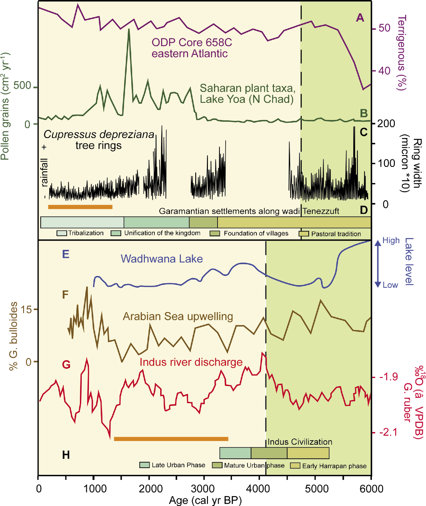
Figure 1: (A) Map with the areas (in green) mentioned in the text (central Sahara and Thar Desert; map: GoogleEarth™). Key: 1) Fazzan (Libya); 2) Thar Desert; 3) Lake Lunkaransar (India); 4) Kotla Dahar (India); 5) ODP Core 658C (off Mauritania); 6) Lake Yoa (Chad); 7) Lake Wadhwama (India). (B) In both regions, the study of subsistence strategies of resilient traditional societies is a tool to disclose the complexity of the responses of late Holocene archaeological communities to increased aridity. |
The African Humid Period is regarded as the most favorable period for human settlement in northern Africa during the Holocene. It corresponds to the so-called Green Sahara, often seen as the apex of Saharan prehistoric civilizations. Its termination represents a crucial moment for past communities. Whether the African Humid Period ended abruptly (e.g. deMenocal et al. 2000) or gradually (Kröpelin et al. 2008) is still discussed. In the SW Fazzan of Libya (Fig. 1), its end (around 5.5 ka BP) determined the rapid decline of natural resources in the climatically sensitive dunes and lowland environments. On the other hand, along the main rivers, which were fed by large aquifers located within the massifs, seasonal water availability persisted for several millennia (Cremaschi and Zerboni 2009). Smaller rivers may have turned into ephemeral streams, or dried out rapidly, but major endorheic watercourses progressively switched into oases, seasonally reactivated by rainfall (Cremaschi et al. 2006). Coeval with North Africa, the Thar Desert (Fig. 1) desiccation began around 6 ka BP (Madella and Fuller 2006), as revealed by the Lake Lunkaransar sediment record, which after some fluctuations dried out by 5.5 ka BP (Enzel et al. 1999). Recent paleoclimatic records from Kotla Dahar, a lake located at the north-eastern edge of the distribution of Indus settlements (Haryana, India), show a general trend towards desertification and higher evapotranspiration between 5.8 and 4.2 ka BP, followed by an abrupt increase in δ18O values and relative abundance of carbonates, indicative of a sudden decrease in Indian summer monsoon precipitations (Dixit et al. 2014).
Aridification and cultural processes
 |
|
Figure 2: Correlation between climatic data and cultural evolution in the Central Sahara and the Thar Desert in the mid-late Holocene. The transition from green to yellow in the background corresponds to the transition toward aridity; the orange bars are phases of unsteady climate. (A) Termination of the African Humid Period according to terrigenous input from the Senegal River (deMenocal et al. 2000); (B) Saharan pollen record from Lake Yoa (Kröpelin et al. 2008); (C) tree rings of Cupressus dupreziana (Cremaschi et al. 2006); (D) cultural evolution of the Garamantian civilization (Mori et al. 2013); (E) Lake Wadhwana fluctuations in the Thar Desert (Raj et al. 2015); (F) record of Arabian Sea upwelling (Gupta et al. 2003); (G) changes in the Indus River discharge (Staubwasser et al. 2003); (H) cultural evolution of the Indus civilization (Dixit et al. 2014). |
Given the diverse physiographic characteristics of the Sahara and the Thar deserts, the climate-driven changes of the landscape likely occurred with different tempi and magnitudes, thus variably affecting past human societies. In both areas, the reconstruction of mid- to late Holocene cultural trajectories is still affected by the patchiness of radiometric data, as well as the scarcity of field-based studies that consider both morpho-sedimentary and archaeological contexts across the region. Nonetheless, during the aridification phase, archaeological evidence in these areas points to continuity of occupation, but with changes in settlement pattern, rather than full-fledged abandonment.
In the SW Fazzan, the transition from the Late Pastoral (5-3.5 ka BP) to the Final Pastoral (3.5-2.7 ka BP) marks the ultimate adaptation to hyperarid conditions and, later, the rise of the Garamantian kingdom (2.7-1.5 ka BP; Mori et al. 2013). According to the most recent paleoclimatic reconstructions (Cremaschi and Zerboni 2009; see also Fig. 2), it seems that the initial phase of the Garamantian kingdom was characterized by a relatively humid environment, whereas the unification of the kingdom period coincided with a clear decrease in rainfall. The end of the Garamantian kingdom occurred a few centuries after the onset of current hyperarid conditions, and was followed by a new tribal population structure and relocation in the landscape (Mori et al. 2013). Therefore, no deterministic correlation between climate or ecological changes and societal collapse can be postulated.
In north-western South Asia, the beginning of the Harappan Civilization (Early Harappan) roughly coincides with the earliest phase of aridification (5.1 ka BP), and the urbanization period (Mature Harappan) develops in spite of the drying trend. Although the end of the Harappan Civilization has often been associated with extreme climatic events, the question is still under debate. A recent study suggests a possible correlation between the 4.1 ka BP drought event and the onset of the de-urbanization period, which started a couple of hundred years later (Dixit et al 2014). However, more than a collapse, the Late Harappan period (3.8-3.2 ka BP) seems to reflect settlement reorganization in consequence to hydroclimatic changes (Giosan et al 2012), with an increased number of small and more dispersed sites that occupied diverse ecological niches. The scale of hydroclimatic stresses probably decreased the resilience of Harappan society, but on its own does not provide a straightforward, deterministic explanation for the transformations in site size, distribution, and interrelationships across the whole area.
The role of an unsteady climate
Climate change has often been invoked as a reason for cultural change, yet human dynamics are not linearly related to climate change. Humans respond to what they perceive as changes in the landscape and in the available resources. Therefore, the transition to aridity in North Africa and north-west South Asia is better interpreted as the transition to a drier, yet oscillating, climate, with marked annual (or few-year lasting) variations in rainfall, and thus in of natural resources. This might have prompted the adoption of flexible and opportunistic strategies to cope with an unpredictable alternation of wet and dry years. Garamantian and Harappan state-like entities, although born and flourished in dry spells, might not have had the level of flexibility necessary to cope with high-frequency climatic variability and its erratic resource availability. The consolidation of centrally controlled socio-economical structures, including resource redistribution networks, resulted in a loss of resilience that ultimately led to a drastic change of the social organization.
The breakdown of these state-like structures, however, did not result in the abandonment of areas, but in the beginning of new socio-economic realities. Humans embraced new settlement strategies for the exploitation of residual and spotted natural resources. Local-scale choices and the accumulated ecological knowledge played a key role in the development of adaptive modes of landscape occupation and socio-cultural practice up to the present day. The oversimplified assumption of “aridity equal to abandonment” should be carefully reconsidered. In many past and current examples, people living in areas that experience aridity trends prefer to readjust and adapt their lifestyle to new conditions rather than abandon their land. How they adapt to new environmental conditions is one of the big issues of current archaeological research in arid lands. Due to the paucity of archaeological investigations directed toward past communities in the Sahara and the Thar deserts, much of the dynamics related to these adaptive strategies still evade our knowledge. Furthermore, in the areas discussed here, the scarcity of data for the post-Garamantian and, to a lesser extent, post-Harappan periods, prevents the construction of robust models describing demographic fluctuations during the late Holocene. Presumably (compared with present-day local adaptations), a more flexible and less-permanent settlement pattern occurred, featuring villages set around water sources (e.g. springs, oases, ephemeral streams). These villages were connected to more mobile, smaller groups adapted to exploit extremely arid areas. The (pre-)historical root of current adaptation to drylands is a key issue to refine our understanding of human dynamics in extreme environments.
affiliations
1Dipartimento di Scienze della Terra “A. Desio”, Università degli Studi di Milano, Italy
2CaSEs - Complexity and Socio-Ecological Dynamics group, Barcelona, Spain
3Department of Humanities, Universitat Pompeu Fabra, Barcelona, Spain
4School of Geography, Archaeology, and Environmental Studies, University of the Witwatersrand, Johannesburg, RSA
5ICREA, Barcelona, Spain
contact
Andrea Zerboni: andrea.zerboniunimi.it
references
Cremaschi M et al. (2006) Holocene 16: 293-303
Cremaschi M, Zerboni A (2009) C R Geosci 341: 689-702
DeMenocal PB et al. (2000) Quat Sci Rev 19: 347-361
Dixit Y et al. (2014) Geology, doi: 10.1130/G35236.1
Enzel Y et al. (1999) Science 284: 125-128
Gasse F (2000) Quat Sci Rev 19: 189-211
Gupta AK et al. (2003) Nature 421: 354-357
Kröpelin S et al. (2008) Science 320: 765-768
Kuper R, Kröpelin S (2006) Science 313: 803-807
Madella M, Fuller DQ (2006) Quat Sci Rev 25: 1283-1301
Manning K, Timpson A (2014) Quat Sci Rev 101: 28-35
Raj R et al. (2015) Palaeogeogr Palaeoclimatol Palaeoecol 421: 60-74
Staubwasser M et al. (2003) Geophys Res Lett 30, doi: 10.1029/2002GL016822
Harvey Weiss
Across the Mediterranean and west Asia, the effects of the 4.2-3.9 ka BP megadrought included synchronous collapse of the Akkadian Empire in Mesopotamia, the Old Kingdom in Egypt and Early Bronze Age settlements in Anatolia, the Aegean and the Levant.
 |
|
Figure 1: Multi-proxy stack display of older, low resolution and more recent Mediterranean westerlies paleoclimate proxy data for 4.2-3.9 ka BP megadrought (and Alpine flooding), with the high-resolution proxies at Mawmluh Cave, India, and Mt. Logan, Yukon. Bars are proxy uncertainty (at two standard deviations) dating. Grey vertical band indicates ca. 300-year period of collapse, abandonment and habitat tracking in eastern Mediterranean and west Asia synchronous with megadrought (M. Besonen and H. Weiss). |
Decadal to century-scale megadroughts are a recently discovered but now well-documented feature of the Holocene. A major and much-discussed example is the abrupt global megadrought and cooling at ca. 4.2-3.9 ka BP (2200-1900 BC), called “4.2 ka BP megadrought” hereafter. Data for this megadrought are derived from analyses of lake and marine sediments, glacial and speleothem cores, and tree-rings. In the eastern hemisphere, these high-resolution proxy records extend across the Mediterranean to east Asia and Australia. The megadrought signal also crossed the African continent, from Algeria and Egypt to South Africa and from the Horn of Africa to the central Sahara and the Gulf of Guinea. In the western hemisphere, the proxy records extend from Greenland and Iceland to the Caribbean, across North America to the Canadian Yukon, and down the western coast of South America from Peru to Patagonia and the Antarctic (Weiss 2015; Zanchetta 2016). Lower resolution proxy data, retrieved by earlier researchers, either failed to note this megadrought or dated it so loosely that synchronous events were obscured (Fig. 1). The newer high-resolution data are, however, virtually impossible to miss or disregard, such that the 4.2 ka BP megadrought has become the focus of volumes of symposia and research conferences annually, alongside scores of journal articles.
For reasons yet unknown, the major global monsoon and ocean-atmosphere circulation systems were deflected or weakened synchronously at 4.2 ka BP, causing major, century-scale precipitation disruptions and failures. The most notable of these global deflections, and the most regionally extensive, are also the most highly resolved in paleoclimate proxy records and are themselves linked to highly resolved regional archaeological records - a captivating and fast-growing research situation!
The very highest resolution records for the 4.2 ka BP megadrought include, prominently, the estimated 30-50% reduction in precipitation delivered by the Mediterranean westerlies in the eastern hemisphere, where they provide for dry-farming and irrigation agriculture across the Aegean, Levant, Anatolia, Mesopotamia, and Iran. Among these highest resolution archives are Mediterranean and Red Sea marine sediment cores, Italian, Albanian and Anatolian lake sediment cores (Weiss 2015), and recently announced Greek and Iranian speleothem cores with sub-decadal sampling intervals.
Synchronous disruptions for the Indian Summer Monsoon are indicated at very high resolution at the Mawmluh Cave (Berkelhammer et al. 2012), with six-year sampling intervals, at paleolake Kotla Dahar (Dixit et al. 2013), and also now at Lake Rara in the Himalayas (Nakamura et al. 2016), each presenting precipitation proxies for the Indian subcontinent and the monsoon’s contribution of 80% of Nile River flow (Welc and Marks 2014). Further east, the trail of high-resolution aridification records extends to Inner Mongolia and to eastern China, where East Asian Summer Monsoon instabilities affected major Late Neolithic settlement systems (Donges et al 2015), and to Australia, where abrupt, dramatic and sustained weakening of the Indonesian-Australian Summer Monsoon is speleothem documented (Denniston et al 2013).
Also impressive are the high-resolution records in the western hemisphere, which include the ice core at Mt. Logan, Yukon (USA), with 10-year sampling intervals. Here, analysis indicates “major enhanced meridional flow coincident with major changes in the Pacific paleorecords of the balance between El Niño and La Niña, suggesting with other records that 4.2 ka BP inaugurated the ‘modern’ ENSO world” (Fisher 2008). Similarly, the annual resolution of Great Basin tree rings indicates severe cooling with “no evidence that treelines have established at these altitudes since before the 2200 BC treeline drop” and “quite possibl[y] that high elevation ecosystems are now responding in a manner unprecedented in approximately 4,200 years” (Salzer et al. 2013). In sum, the high-resolution data now available indicate that this was a unique and global Holocene climate event second only to the 8.2 ka BP event in magnitude, but perhaps twice its duration. Hence, the onset of the 4.2 ka BP megadrought has been proposed to mark the middle to late Holocene transition (Walker et al 2012).
Societal collapse, regional abandonments and habitat tracking
How did societies adapt to what was a 200-300 year mid-Holocene megadrought? The proxy records for the interruption of the Mediterranean westerlies and the Indian Summer Monsoon are located where regional archaeological records are most numerous and highly resolved: the Mediterranean, the Levant, Egypt, Turkey, and Mesopotamia. Here, widely distributed and organizationally different, cereal-agriculture-based societies collapsed synchronously and coincident with the megadrought. The archaeological record for these societal collapses includes (1) intensive regional settlement surveys (2) high-resolution radiocarbon dating for abrupt abandonments in dry-farming domains across the scales of settlement, from villages to cities, and (3) epigraphic and radiocarbon data for the collapses of the region-wide, expanding Mesopotamian Akkadian Empire and the Nile-based Egyptian Old Kingdom (Ramsey et al. 2010; Weiss et al. 2012; Davis 2013).
 |
|
Figure 2: Syria and Mesopotamia, 4.2-3.9 ka BP, indicating major dry-farming settlement abandonments and reductions and habitat tracking to riparian, paludal and karstic refugia (S. Maples and H. Weiss). |
In these regions dependent upon rain-fed agriculture, the adaptive societal response linked with abandonment was habitat-tracking to riparian, paludal and karstic refugia. Region-wide settlement surveys suggest that the populations abandoning the rain-fed plains of southwestern Turkey, western Syria and northern Mesopotamia became the habitat-tracking populations that settled along the banks of the Euphrates River and the karst-spring fed Orontes River (Fig. 2). Similar habitat tracking occurred synchronously in the southern Levant and in the western Mediterranean.
Pastoralist adaptations
The Amorites, a large tribal confederation of pastoral nomad “campers”, also exploited the Mesopotamian and Levantine landscapes, traversing the middle Euphrates River valley seasonally to steppe lands and dry-farming plains for sheep-flock forage. The abrupt desiccation disrupted this ancient seasonal pattern, forcing the tribal groups to seek refugia along and down the Euphrates River. This infiltration of southern Mesopotamian urban kingdoms prompted their dynasts to construct the “Repeller of the Amorites” wall recorded in contemporary records. The wall proved porous, however, and within a few generations the former pastoralists’ descendants became the Amorite rulers of Babylon. Indeed, the megadrought at 4.2-3.9 ka BP, serendipitously the best-documented period in cuneiform sources for southern Mesopotamia, was previously understood to represent inherently maximizing irrigation-based agriculture and hypertrophic city growth. But its anomalous character, a function of demographic and subsistence forces unleashed by the 4.2 ka BP megadrought, now encourages environmental historicization.
What caused the resettlement?
An explanation for the resettlement of Mesopotamian dry-farming domains, and the opportunistic sedentarization of formerly pastoralist Amorites at the abrupt ca. 1900 BC return of pre-aridification precipitation, now comprises a major anthropological and archaeological challenge, even though the historical moment is well-documented. The resettlement swiftly generated the famous warring kingdoms associated with the empire of Shamshi-Adad of Assyria and massive military struggles for rain-fed land and imperial power across west Asia. Resettlement is apparently not self-evident: for instance, the post-megadrought abandonment of the central Maya Lowlands in the 9th century AD continued.
Similarly, the variabilities within several other Holocene societal collapses are now available for cross-cultural exploration, including the 3.2 ka BP megadrought that caused Mediterranean and west Asian collapses and resettlements; the megadrought-induced 11th century AD collapse of the Tiwanaku state and its raised–field agriculture at Lake Titicaca in western Bolivia and subsequent highland-lowland habitat tracking; the synchronous Wari empire collapse in Peru that was followed by the Late Intermediate Period surge of warfare, elevated morbidity and excess mortality; the 13th century AD “Great Drought” and Ancestral Pueblo regional abandonments and habitat tracking to refugia in southwest North America; and the collapse and abandonment of the expansive “hydraulic city” at Angkor, Cambodia, following 13th-14th century AD decadal droughts and high-magnitude monsoons.
Future research
As a new generation of researchers amass high-resolution data for megadrought and societal responses at 4.2 ka BP, developing research arenas include Greece and the southern Levant, where the megadrought data are certain but some regional archaeological surveys remain insufficiently resolved; the Indus Valley, where the paleoclimate data are also clear but archaeological periods require better dating; China, where northern regions were desiccated and abandoned (Yang et al. 2015) while Yellow River extreme flooding is reported during Longshan-period urban collapse; North America, where the megadrought is close in time and space with the earliest crop domestication in the Yucatan and eastern North America, thereby challenging current origins of agriculture hypotheses; and Peru, where the 4.2 ka BP event may have conditioned abandonment of the Late Pre-ceramic Supe Valley cities (Weiss 2015).
Societal resilience
The multi-century 4.2 ka BP megadrought generated adaptive societal collapse, abandonment and habitat tracking across hydrologically varied landscapes. These proved to be resilient strategies for the diverse peoples and polities of the Mediterranean and west Asia. Previously mysterious and unexplained, these synchronous ancient events are now historical processes linking dynamic societies and abrupt Holocene megadrought. Moreover, the evidence prompts further proxy resolution, modeling and explanation.
affiliation
School of Forestry and Environmental Studies, Yale University, New Haven, USA
contact
Harvey Weiss: harvey.weissyale.edu
references
Davis J (2013) Am J Arch 117: 527-533
Denniston R et al (2013) Quat Sci Rev 78:155-168
Dixit Y et al. (2014) Geology 42: 339-342
Donges et al (2015) Clim Past 11: 709–741
Fisher D et al. (2008) Holocene 18: 667-677
Nakamura A et al. (2016) Quat Int 397: 349-359
Ramsey CB et al. (2010) Science 328: 1554-1557
Salzer MW et al. (2013) Clim Dyn 42: 1517-1526
Walker M et al. (2012) J Quat Sci 27: 649-659
Welc F, Marks L (2014) Quat Int 324: 124-131
Julio L. Betancourt1 and Christopher H. Guiterman2
Chaco Canyon was the center of a regionally integrated system. Despite a century of research, questions remain about its rise and fall, and the role of human-environment interactions. The answers may lie in current events and new tools and perspectives.
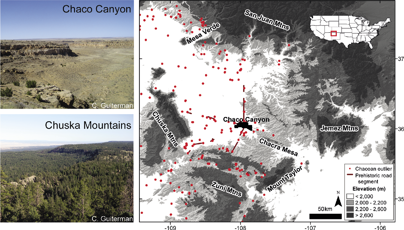 |
|
Figure 1: The regional system centered on Chaco Canyon, but associated “outlier” communities populated the western half of the San Juan Basin. Distant areas like the Chuska Mountains were far richer in timber and other resources than Chaco Canyon at the time, as they are now. |
Chaco Canyon in northwestern New Mexico, USA, boasts a spectacular array of prehistoric ruins, meriting status as a US National Historical Park and UNESCO World Heritage Site. First excavated 120 years ago, Chaco Canyon may be the most-studied archaeological site in the USA, motivating hundreds of publications and even its own queryable archive and database (www.chacoarchive.org/cra/). The desolate canyon, a marginal and unpredictable environment, supported the Ancient Puebloans in developing a complex society and regionally integrated system that, at its nadir in the 11th century, was centered on Chaco and spanned >50,000 km2 (Fig. 1). In popular literature, Chaco’s genesis inspires awe - “a dazzling show of wealth and power in a treeless desert” (Fernández-Armesto 2001) - while its collapse stirs deep reflection about “environmental impact and climate change intersecting” (Diamond 2005).
Despite more than a century of focused research, there are still many unanswered questions (e.g. Plog and Heitman 2010). The Chaco Phenomenon emerged quickly ~AD 850 from dispersed rural communities subsisting on maize, beans and squash, flourished for a few centuries, then collapsed between AD 1130 and 1150. In its heyday, the Chaco Phenomenon was distinguished by planned architecture of multistoried great houses; shared ceramic traditions and rituals; intensive agriculture and sophisticated water-control features; long-distance trade of luxury items (cacao, macaw and parrot feathers, copper bells, turquoise, and seashells); and an extensive network of well-constructed roads.
Integrating a regional human-environmental system
Today, Chaco is deficient in natural resources (Fig. 1), giving rise to the idea that Chaco Society was a regionally integrated system that relied on resource-rich areas and outlying communities. Chaco could have acted as a center for storage and redistribution of surplus food, particularly maize, by a small and elite population housed in the canyon, or as a religious center into which food and other goods flowed during pilgrimages that reinforced system-wide religious authority. Others counter that Chaco looked very different 1,000 years ago, and was a productive agricultural center able to sustain a large population throughout most of its three-century tenure. These differing perspectives on the Canyon’s environment and its social structure lead to widely ranging population estimates during the Chaco Phenomenon, from <10,000 to >100,000 people (Minnis 2015).
Timber and fuel for great houses
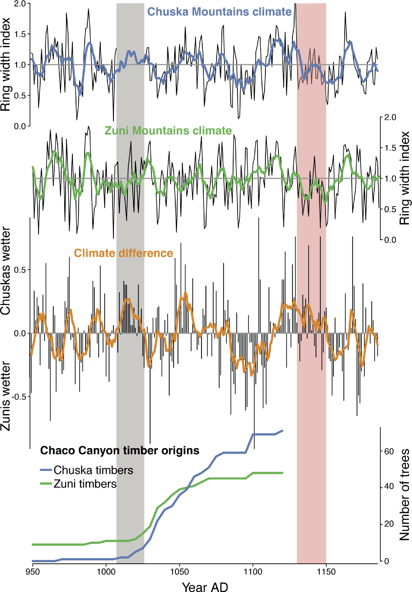 |
|
Figure 2: Local climates and timber extraction. Precipitation-sensitive tree-ring-width chronologies from the Chuska and Zuni Mountains show sub-regional differences in the timing, duration and severity of drought. One period (AD 1007-1026; grey shading) coincides with the arrival of Chuska timbers to Chaco Canyon. The 12th century megadrought (AD 1130-1150; red shading) probably initiated collapse at Chaco and was longer and deeper in the Chuskas than the Zunis. Bold lines in the top three panels are seven-year running averages. The third panel shows the difference between the Chuska and Zuni tree-ring chronologies. Data from Guiterman et al. (2016). |
The Ancient Puebloans at Chaco quarried sandstone blocks and logged hundreds of thousands of trees, mostly big conifers that do not grow locally today, to build the dozen or more great houses, considered the largest buildings in North America north of Mexico until the 19th century. Plant macrofossils from packrat middens on the canyon slopes showed that ponderosa pine (Pinus ponderosa), the main architectural timber, grew locally only as scattered individuals during the late Holocene - not enough to sustain architectural needs (Betancourt and Van Devender 1981). Engelmann spruce (Picea engelmannii) and subalpine fir (probably Abies lasiocarpa), which made up a quarter of the architectural wood (Betancourt et al. 1986), last grew in the canyon 12,000 years ago, and must have been logged from mountaintops >75 km away. Tree-growth patterns show that, prior to AD 1020, nearly all of the timber was procured from the Zuni Mountains >80 km to the southwest (Guiterman et al. 2016). Later during the mid-11th century Chacoan fluorescence, both tree-growth patterns and strontium isotopes indicate that most of the timber came from the Chuska Mountains >75 km to the west (English et al. 2001; Reynolds et al. 2005; Guiterman et al. 2016). This shift in tree sources is associated with nearly two decades of drought conditions in the Zunis that were apparently less marked in the Chuskas (Fig. 2). Along with timber, the Chuskas were a major source for stone tools, pottery and maize. The area also emerges as a primary resource for deer, rabbits and prairie dogs consumed at Chaco (Grimstead et al. 2016).
While timber and other resources were clearly procured from long distances, fuelwood was available locally. The packrat midden record shows persistent and ubiquitous pinyon pine throughout the late Holocene until it was locally extirpated between AD 700 and 1500. To this day, pinyon populations show no sign of recovery. So the question is not just what caused pinyon’s extirpation, but also what has prevented its recovery? The explanation could well involve climate or woodcutting. Under a woodcutting scenario (Samuels and Betancourt 1982), Chacoans could have easily wiped out the woodland in a couple centuries, likely pushing firewood gathering to more distant stands, including nearby Chacra Mesa. Ultimately, this could have reduced nearby seed sources from which local pinyon populations could regenerate.
A possible role for megadrought
Impacts of the recent 2000s drought in the region underscore a climate explanation. Over the last two decades, severe droughts in western USA have resulted in widespread and synchronized ecological disturbances, including wildfires, pine beetle outbreaks, and tree die-offs (Williams et al. 2013). These events have inspired a flurry of research on the impacts of hotter drought associated with anthropogenic warming, but both archaeologists and paleoecologists, including the authors, are currently revisiting the enigmatic ecological footprints of past droughts. Could pinyon at its lower and dry limits in Chaco Canyon have been wiped out by the mid-12th century megadrought? Occurring during the height of the unusually dry Medieval Climate Anomaly (MCA; AD 900-1300), the mid-12th century megadrought far exceeded the severity, duration and extent of subsequent droughts (Woodhouse et al. 2010). Although ecological impacts are less well-documented, we do know that this, and other MCA droughts, synchronized extensive wildfires from California (Swetnam et al. 2009) to Colorado (Calder et al. 2015). It is likely that these droughts also produced widespread tree die-offs. As part of an ongoing study to assess past ecological disturbances in the Chuska Mountains, one of us (CHG; unpublished data) sampled over 1000 trees and found only eight that were established before AD 1150, with just three trees surviving the mid-12th century megadrought, which was apparently more severe in the Chuskas than in the Zuni Mountains to the south (Fig. 2).
Future questions
Did impacts of the extended mid-12th century drought in the Chuskas have a cascading effect on the Chaco Core and its regional system? Was the shift in sources of architectural timber from the Zuni to the Chuska Mountains around AD 1020 driven by asynchroneity in hydroclimate variability across the region, perhaps related to shifting epicenters of droughts and pluvials? Did sub-regional syn- and asynchroneities in climate and ecosystems, perhaps changing over time, determine Ancestral Puebloan movements initially to Chaco and later to other sites during abandonment? This is precisely the modeling approach taken by Bocinsky and Kohler (2014) in using tree-ring data to model the rain-fed, maize agricultural niche across the US Southwest. The same could be done for other essential resources, which could have shifted dramatically with large and synchronized disturbances driven by drought. Although Chaco Canyon has been well studied, most of the excavations and the published literature happened in the 20th century. The prospects for new research at the intersection of human impacts and climate change are not only exciting but in order.
affiliations
1US Geological Survey, Reston, USA
2Laboratory of Tree-Ring Research, University of Arizona, Tucson, USA
contact
Julio L. Betancourt: jlbetancusgs.gov
references
Betancourt J et al. (1986) American Antiquity 51: 370-375
Betancourt J, Van Devender T (1981) Science 214: 656-658
Bocinsky R, Kohler T (2014) Nature Comm 5, doi:10.1038/ncomms6618
Calder W et al. (2015) PNAS 112: 13261-13266
Diamond J (2005) Collapse: How Societies Choose to Fail or Succeed, Penguin Books, 571 pp
English N et al. (2001) PNAS 98: 11891-11896
Grimstead D et al. (2016) Geoarchaeology, doi: 10.1002/gea.21545
Guiterman C et al. (2016) PNAS 113: 1186-1190
Plog S, Heitman C (2010) PNAS 107: 19619-19626
Samuels M, Betancourt J (1982) Environ Manage 6: 505-515
Swetnam T et al. (2009) Fire Ecol 5: 120-150
Tim Beach1, S. Luzzadder-Beach1, N. Dunning2 and D. Cook3
Archaeology and paleoclimatology provide insights into the vagaries of Maya history and climate. Although millions of Maya persist today, three main historical declines coincide with drought records. These are important examples of humanity’s complex interactions with drought and environmental change.
The idea that the Classic Maya of Central America “collapsed” dates back to at least the 19th century (Luzzadder-Beach et al. 2012). Explorers like Stephens and Catherwood, in the 1840s, documented many ancient Maya cities in stages of decay. These writings and pictures of temple ruins enshrouded by tropical forest provided imagery of a lost Maya world. Both “collapses” (profound reductions in population or reductions in social complexity) and “declines” (depopulations) occurred over Maya history. Archaeologists have long studied both, and the roles that climate may have played has attracted worldwide attention, but how this great culture persisted is even more interesting (Beach et al. 2015). Although there is convincing paleoclimatic evidence for droughts during several Maya periods, the archaeological evidence for collapse during any of these periods remains coincidental.
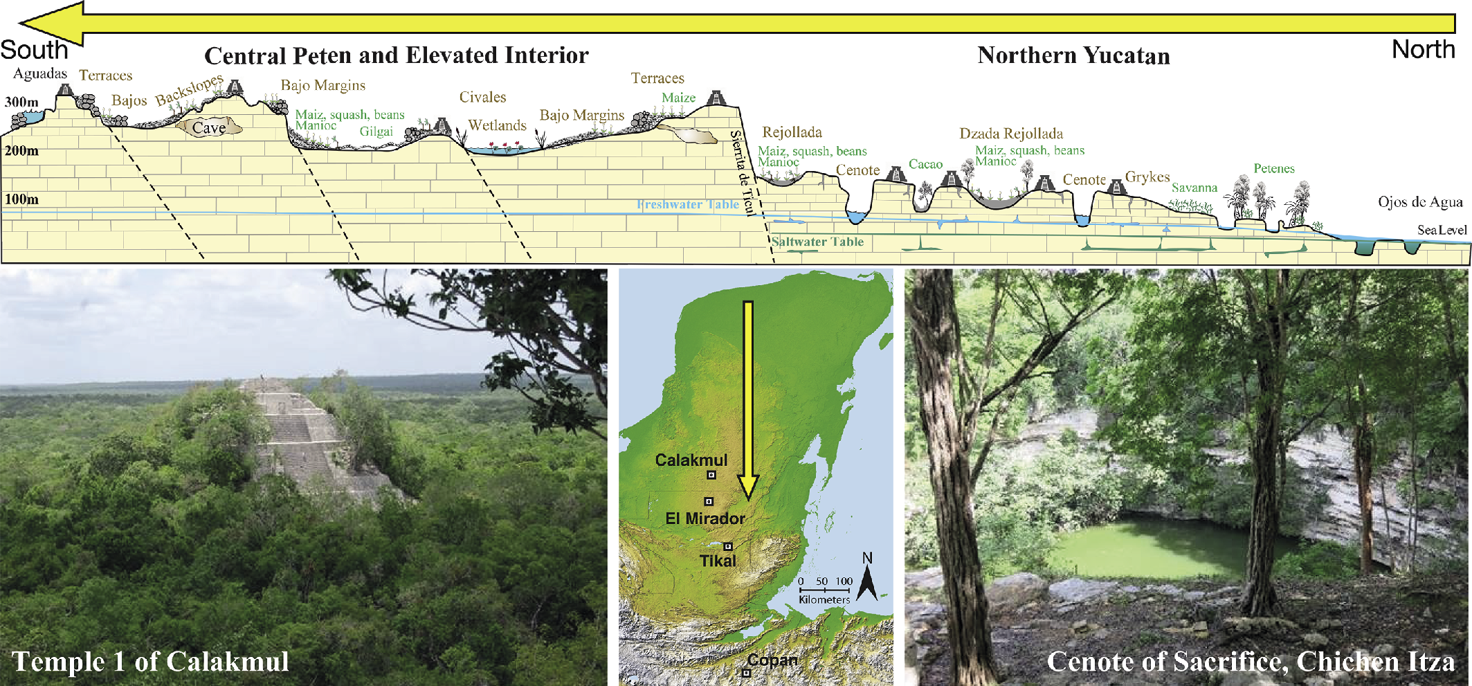 |
|
Figure 1: Map and landscape diagram of the Yucatán Peninsula in Central America showing the relationship between the Maya lowlands and the more elevated interior. |
The vagaries of Maya cities varied across time and space. In the northern Yucatán, the city of Mayapán collapsed around 1440 AD and Chichén Itzá declined around 1250 AD. The Maya heartland cities from Uxmal southward to Copán flourished into the 9th and 10th centuries AD (Fig. 1). El Mirador and other early urban centers collapsed much earlier, around 150 AD. These lines of evidence suggest three main cessation periods: The Late Preclassic (300 BC-250 AD) or just after, the Late and Terminal Classic (700-1000 AD), and the Early Post Classic (1000-1100 AD). Several paleoclimate records indicate drier conditions either during or near these three periods of social and cultural upheaval (Fig. 2), and some studies linked the Middle Classic hiatus, a period of stagnation (ca. 550 AD) around Tikal, to drought (Beach et al. 2015).
But scholars debate when collapse actually occurred or if any specific collapse occurred because millions of Mayan language speakers still exist. One view is that the collapse occurred mainly after European conquest and subsequent indigenous population declines, caused by European diseases, forced religious and social conversions, and cultural truncation. One vivid example of this was Europeans burning Maya books, terminating a millennia-old glyph-based language.
 |
|
Figure 2: Climate proxy records overview for the Maya lowlands with droughts highlighted in yellow (redrafted after Luzzadder-Beach et al. 2016). See text for references to numbers in the right-hand column. |
A key region of Maya lowlands collapse was the Elevated Interior Region (EIR), which lies prone to water stress far above perennial water sources. Here the Maya built various forms of water storage such as the many reservoirs at the great cities of Tikal and Caracol (Beach et al. 2015). The Maya tended to overbuild reservoirs to withstand rainfall variability, but these systems may not have been survivable under severe droughts. Indeed, the EIR was an appealing place in the wetter Preclassic and drought remained manageable even in the drier Late Preclassic, but later droughts may have proved insurmountable (Fig. 2).
The Maya Collapse literature includes a legion of causes, such as droughts, soil deterioration, hurricanes, epidemics, and seismicity, as well as social upheavals in religion, warfare, and trade routes (Beach et al. 2015). Climate change could have led to crop failures, famine and refugees. These in turn could have led to other environmental or social changes, like the Maya rejection of rulers, warfare or changes in trade routes away from the EIR, which could never regenerate in this drought-prone land (Turner and Sabloff 2012).
Like other tropical climates, the Maya lowlands has pronounced wet and dry seasons. The May through November wet season arises from atmospheric instability of the intertropical convergence zone (ITCZ) and the December to May dry season is caused by air stability from the subtropical high pressure (STHP). Rainfall comes from convection and convergence systems of all scales and varies both inter-annually and geographically, ranging from 500 mm per annum in northwest Yucatán to above 3000 mm in the southern mountains (Fig. 1).
The Maya lowland’s climate change record derives from cave speleothems, and lake and marine sediments (Fig. 2). Speleothem records are especially important because of their finer chronology that can overlap with instrumental records. Speleothems that can accurately fit instrumental records provide confidence for hindcasting past climate and overlapping the many but coarser-resolved lake records.
These records indicate three key arid periods that coincide with declines of Maya polities. The earliest such drought occurs in the last century of the Late Preclassic (150-250 AD), and three northern Yucatán and southern Belize speleothem records indicate drought at or just after this time (Fig. 2.1, 2.2, 2.3). Sediments from the northern Yucatán lakes and the Cariaco Basin provide overlapping evidence (Figure 2.4, 2.6, 2.7, 2.8). The archaeological evidence includes the collapse of the giant site of El Mirador and allied centers, as well as the iconic Preclassic site of San Bartolo and coastal site of Cerros (Fig. 1), but elsewhere there were mainly temporary declines and social upheavals (Dunning et al. 2012; Iannone 2014). A speleothem record from the heart of the collapse zone in Guatemala’s Petén may help us frame this drought.
The Middle Classic hiatus (ca. 550 AD) provides a less-convincing case. Studies from around the world indicate a global cooling event (Büntgen et al. 2016) and at least two large volcanic eruptions (one possibly from Mesoamerica) from 536-540 AD (Sigl et al. 2015). Some studies link drought and cultural declines at this time, but most link the hiatus with war mainly around the Tikal region (Iannone 2014).
The Terminal Classic saw the decline of many more cities, ranging spatially from Yucatán to Honduras and temporally from about 700 to 900 AD (Webster 2002). A few cities, especially coastal plain or riverine ones like Lamanai, flourished longer (Beach et al. 2015). The climatic evidence also has a wide geographic range from northern Yucatán to the Cariaco Basin, though some records are more equivocal (Fig. 2). One key climate archive has been Laguna Chichancanab (Fig. 2.4, 2.7; Hodell et al. 1995), where the scientific study of the Terminal Classic drought began (Beach 2016). Several climate records also indicate droughts in the Early Post Classic (Fig. 2.1, 2.2, 2.5, 2.7).
Some research also suggests the Late-Terminal Classic drought period had more extreme events like hurricanes, which could have exacerbated drought impacts and masked their severity (Frappier 2013). Indeed, the Maya dealt with overlapping hazards in the Late- and Terminal Classic. Hurricane runoff can damage soils and trees and lead to an increased risk of forest fire from fuel build-up. Sea-level rise affected many coasts, and the lack of large coastal Maya cities suggests coastal hazards played some role in ancient Maya urban geography (Dunning et al. 2012).
The Terminal and Postclassic droughts would have been challenging to any civilization, and especially so in the Maya heartland with its dearth of permanent water sources. Some studies suggest that the Maya here started building reservoirs in the Late Preclassic and Early Classic coincident with or after drought, which may have offered stability for centuries. But sedimentation reduced storage capacity so that by the intense droughts of the Late to Post Classic water storage (resiliency) had diminished (Beach et al. 2015). Also, the large-scale abandonment of the Terminal Classic may have reset Maya trade and production geography, which the Early Postclassic drought reinforced. More droughts occurred later in the Little Ice Age and the long trend of Late Holocene drying (Wanner et al. 2008) may have made the EIR unattractive. Thus, the EIR, erstwhile center of Maya Civilization, lost its appeal by the Postclassic. Thereafter, the Maya chose to live, trade and farm near perennial water sources along the Maya lowlands’ margins until European conquest.
The 21st century is bringing new climate challenges to the Maya lowlands. The IPCC anticipates that temperatures will rise and precipitation fall, increasing water stress (Margrin et al. 2014). We still need more research that can pair climate histories with archaeology to better understand the role of climate in Maya history. New paleoclimate research from this data-poor region can complement and extend modern records of climate and improve models of future climate change. Likewise, archaeological research that can identify and date features that signify adaptation to droughts, like dams, canals and water harvesting, may help us identify critical thresholds in social responses to water stress.
affiliations
1Geography and the Environment, The University of Texas at Austin, USA
2Geography, The University of Cincinnati, USA
3School of Arts, Australian Catholic University, Brisbane, Australia
contact
Tim Beach: beachtaustin.utexas.edu
references
Beach T et al. (2015) Quat Sci Rev 124: 1-30
Beach T (2016) Global Planet Change 138: 1-2
Büntgen U et al. (2016) Nat Geosci 9: 231-236
Dunning N et al. (2012) PNAS 109: 3652-3657
Frappier AB (2013) Geochem Geophys Geosyst 14: 3632-3647
Hodell DA et al. (1995) Nature 375: 391-394
Luzzadder-Beach S et al. (2012) PNAS 109: 3646-3651
Luzzadder-Beach S et al. (2016) Antiquity 90: 426-442
Sigl M et al. (2015) Nature 523: 543-549
Turner BL, Sabloff JA (2012) PNAS 109: 13908-13914