PAGES Magazine articles
Tim Brücher1, V. Brovkin1, S. Kloster1, J.R. Marlon2 and M.J. Power3
An Earth system model of intermediate complexity and a land surface model are used to simulate natural fire activity over the last 8000 years. We demonstrate the benefits of using Z-scores as a metric for validating model output with transformed charcoal records.
Fire is an important process that affects climate through changes in CO2 emissions, albedo, and aerosols (Ward et al. 2012). Fire-history reconstructions from charcoal accumulations in sediment indicate that biomass burning has increased since the Last Glacial Maximum (Power et al. 2008; Marlon et al. 2013). Recent comparisons with transient climate model output suggest that this increase in global fire activity is linked primarily to variations in temperature and secondarily to variations in precipitation (Daniau et al. 2012).
Methodology
In this study, we discuss the best way to compare global fire model output with charcoal records. Fire models generate quantitative output for burned area and fire-related emissions of CO2, whereas charcoal data indicate relative changes in biomass burning for specific regions and time periods only. However, models can be used to relate trends in charcoal data to trends in quantitative changes in burned area or fire carbon emissions. Charcoal records are often reported as Z-scores (Power et al. 2008). Since Z-scores are non-linear power transformations of charcoal influxes, we must evaluate if, for example, a two-fold increase in the standardized charcoal reconstruction corresponds to a 2- or 200-fold increase in the area burned. In our study we apply the Z-score metric to the model output. This allows us to test how well the model can quantitatively reproduce the charcoal-based reconstructions and how Z-score metrics affect the statistics of model output.
The Global Charcoal Database (GCD version 2.5; https://www.paleofire.org/index.php) is used to determine regional and global paleofire trends from 218 sedimentary charcoal records covering part or all of the last 8 ka BP. To retrieve regional and global composites of changes in fire activity over the Holocene the time series of Z-scores are linearly averaged to achieve regional composites.
A coupled climate–carbon cycle model, CLIMBA (Brücher et al. 2014), is used for this study. It consists of the CLIMBER-2 Earth system model of intermediate complexity and the JSBACH land component of the Max Planck Institute Earth System Model. The fire algorithm in JSBACH assumes a constant annual lightning cycle as the sole fire ignition mechanism (Arora and Boer 2005). To eliminate data processing differences as a source for potential discrepancies, the processing of both reconstructed and modeled data, including e.g. normalization with respect to a given base period and aggregation of time series was done in exactly the same way. Here, we compare the aggregated time series on a hemispheric scale.
Modeled fire activity vs. reconstructions
 |
|
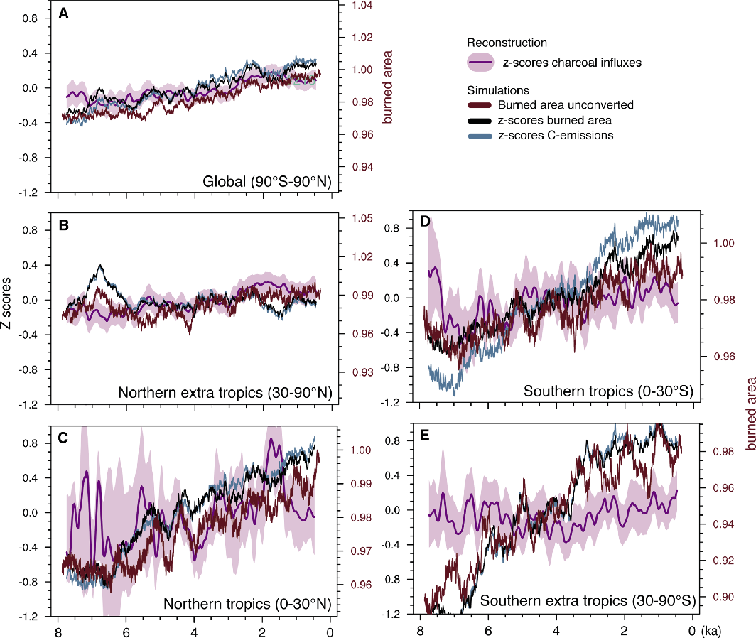
Figure 1: Reconstructed and modeled biomass burning over the last 8 ka. Curves represent zonal averages smoothed with a 250-year running mean on global (A), extra tropical (B, E) and tropical (C, D) scales. Reconstructions are shown by Z-scores of charcoal influxes (pink). Model output is given by untransformed burned area (brown) and by the Z-score transformed values of modeled burned area (black) and fire-related carbon emissions (blue). |
We simulate a global increase of approximately 3% (from 512 to 526 Mha) in burned area over the past 8 ka (Fig. 1A). The burned area is high against present day observations. The model only accounts for fire activity involving natural vegetation because it ignores land use effects. The gradual increase of burned area and the variability on millennial timescales differ between and among regions; however, the modeled time series transformed to Z-scores and the reconstructed charcoal Z-scores agree well within most of the hemispheric regions , except the Southern extra tropics which are dominated by the ocean and therefore only few model grid boxes are available to compare with. Thus, we can state that our model simulates most of the trends in the fire activity reconstructions on millennial scales.
Z-score transformed data do not provide quantitative information about changes in burned area, because the transformation is rank-conserving but not linear. A given difference in Z-score values does not imply the same magnitude in Mha of burned area among Z-scores from a different time interval or region. This suggests that regional averages of transformed and untransformed data may not necessarily result in the same trends. For example two sites with opposite trends e.g. +50% (from 20Mha to 30 Mha) and -50% (from 100 Mha to 50 Mha) would be merged to a constant Z-score of fire activity, in spite of a decrease in the absolute area burned. Thus, with respect to our research question we conclude that it is more meaningful to convert the time series of modeled burned area or carbon emissions to Z-scores for comparing modeled and observed paleofire variability than comparing quantitative data by the model with qualitative trends out of reconstructions. While we do see some general agreement between model results and reconstructions, it is still unclear whether the absolute values of simulated burned area are capturing the right magnitude of past fire activity.
In all regions, the trends in simulated fire-related carbon emissions are higher than trends in simulated burned area (Fig. 1). We propose several reasons for this observation: (i) increasing atmospheric CO2 over the Holocene leads to a higher level of CO2 fertilization. The resulting higher level of carbon stock in the vegetation results in higher emissions per square meter of area burned. (ii) The carbon stock of the fuel can increase with shifts in vegetation type, e.g. from grassland to forest, due to changing climate, or (iii) fire occurrence may be altered by changes in dryness due to climate changes. A rank correlation analysis points to an overall agreement between simulated and observed trends in fire activity over the whole study period, while the rank correlation on 4000-year time segments shows that the model does not match the centennial- or millennial-scale variability (not shown). Model-data agreement on fire variability on these centennial timescales is not necessarily expected. Regional climate affects local fire activity, and due to internal variability there is no reason why the timing of modeled fire events should coincide with the reconstructed timing.
Summary
This study provides a method for validating a model’s capability to simulate past fire activity. Given that our fire model is not tuned by any charcoal data, the overall data-model agreement within climatic zones validates the paleofire activity reconstructions from syntheses of paleofire records in the Global Charcoal Database. Even regions that are sparsely covered by reconstructions correlate positively with the model results. This points to the benefit of using both data and models together to provide more complete spatial coverage of past fire activity.
Further investigations are necessary to test whether the model performs well for the right reasons. If the driving factor for a reconstructed fire trend is known, the factor separation approach can be applied to test the underlying fire algorithm (Kloster et al. 2014). Despite the great work to synthesize all available charcoal records for regional trends, the information is currently limited to quantitative trends, Future studies on model-data comparison should therefore consider transforming model output variables and paleo-proxy data consistently to improve the comparability of simulated and observed data. In this study, we found that the Z-score transformation helped to validate modeled fire occurrence and compare it to charcoal records. From a modelling perspective it would be preferable to get also quantitative information such as type of biomass burning and area burned).
affiliations
1Max Planck Institute for Meteorology, Hamburg, Germany
2School of Forestry and Environmental Studies, Yale University, New Haven, USA
3Natural History Museum of Utah, Department of Geography, University of Utah, Salt Lake City, USA
contact
Tim Brücher: tim.bruecher mpimet.mpg.de
references
Arora VK, Boer GJ (2005) J Geophys Res 110, doi:10.1029/2005JG000042
Brücher T et al. (2014) Clim Past, 10: 811-824
Daniau A-L et al. (2012) Global Biogeochem Cycles 26, doi:10.1029/2011GB004249
Kloster S et al. (2014) Clim Past Discuss, doi:10.5194/cpd-10-4257-2014
Marlon JR et al. (2013) Quat Sci Rev 65: 5-25
Marlon JR et al. (2009) PNAS 106: 2519-2524
Power M et al. (2008) Clim Dyn 30: 887-907
Ward DS et al. (2012) Atmos Chem Phys 12, doi:10.5194acp-12-10857-2012
Pepijn Bakker1,2, A. Govin3, D. Thornalley4, D. Roche1,5 and H. Renssen1
Using a climate model we investigate how changes in the strength of the Atlantic Meridional Overturning Circulation (AMOC) are reflected in water flow speeds and foraminiferal δ13C, two tracers of AMOC variability commonly measured in marine sediment cores.
Investigating past changes in the Atlantic Meridional Overturning Circulation (AMOC) provides us with clues about the possible multi-decadal to centennial response of the AMOC to projected global warming. Realistic and physically consistent evidence about past changes can be obtained from combining ocean model simulations of past scenarios with real-world proxy data. The common approach for this is to qualitatively compare the model output, i.e. the simulated stream function of maximum AMOC with paleocanographic reconstructions, e.g. foraminiferal δ13C as a proxy for deep sea ventilation changes (Duplessy 1981; Shackleton 1977), or sortable silt as a proxy for bottom water flow speed (McCave et al. 1995). However, this approach is limited to being semi-quantitative at best because (i) different paleoceanographic proxies record different aspects of the AMOC and (ii) comparing these proxies to climate model outputs is not trivial since non of the proxies record the physical overturning as expressed by the stream function. We therefore simulated the water flow speed and δ13C directly within the ocean circulation model. This allows us to discuss what aspects of AMOC changes the two AMOC proxies record, and how this depends on the geographical context.
Towards more direct model-data comparisons
Full carbon cycle dynamics, including isotopes, have been developed and built into the 3-dimensional global climate model of intermediate complexity, iLOVECLIM (Bouttes et al. 2014). In our study, we focus on the Last Interglacial period (LIG; ~130-116 ka BP), which is particularly relevant to future concerns because it was characterized by significant changes in the AMOC strength (Galaasen et al. 2014, and this issue; Govin et al. 2012; Hodell et al. 2009; Oppo et al. 1997, 2006; Sânchez-Goñi et al. 2012) at global temperatures higher than today (e.g. CAPE Members 2006).
We performed a fully coupled transient simulation that covers the 132-120 ka BP time interval. We mimicked the range of reconstructed AMOC changes by gradually tuning up its strength in the model from a nearly collapsed state, to a weak state, and finally, a strong state similar to the present-day. Accordingly, the model produced changes in flow speed and δ13C.
 |
|
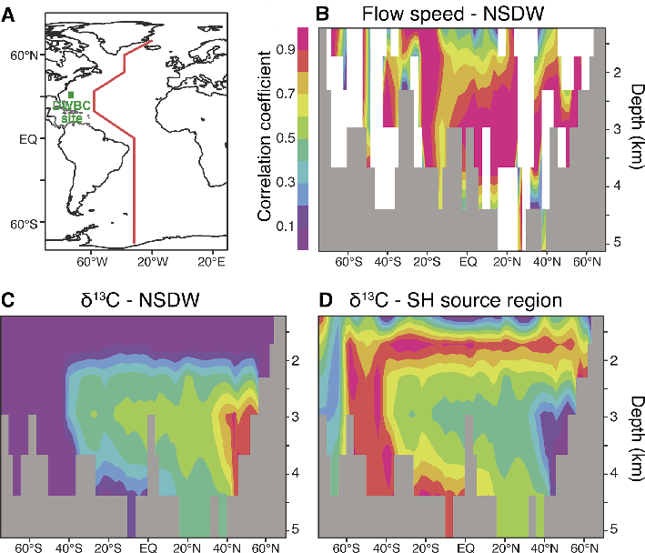
Figure 1: Correlations between AMOC driving factors and simulated flow speeds or δ13C along a vertical transect through the Atlantic. (A) Map showing the transect path (red line) and the site used in Fig. 2 (green rectangle). (B) Correlations of the flow speed with NSDW. Correlation of δ13C with (C) NSDW, and (D) SH-source region δ13C changes. The cross-section roughly follows the western boundary of the Atlantic basin. Gray shading means bottom topography; white shading means that no linear combination of the drivers yielded a correlation with the flow speed changes above 0.5. |
 |
|
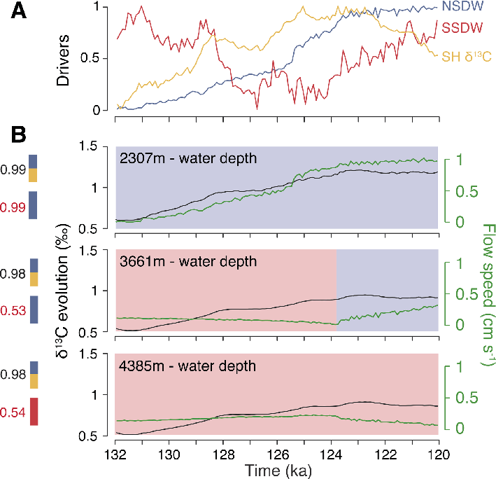
Figure 2: Comparison of the simulated evolution of AMOC indicators during the LIG and their main large-scale drivers for three water depth levels at a site (grid-cell) located in the path of the DWBC in the subtropical northwestern Atlantic (green rectangle in Fig. 1A). (A) Simulated main drivers. (B) Evolution of δ13C (black) and flow speed (green). The vertical colored bars and associated R2 correlation values indicate the relative importance of the main (normalized) drivers shown in panel A in reaching a best linear fit with the simulated records of δ13C (top bar) and flow speed (lower bar), respectively. For flow speed only NSDW and SSDW were taken into account. Red and blue shading of the panels indicate the water mass prevalent at each depth level, where southward flow was taken to be indicative of SSDW, northward flow of NSDW. |
To constrain the underlying mechanisms of flow speed and δ13C we calculated temporal correlations with several potentially important drivers. For local flow speed changes we consider two potential drivers: the transport of deep water formed in the North Atlantic (northern-sourced deep water; NSDW) and deep water formed in the Southern Ocean (southern-sourced deep water; SSDW). In addition to the transport of NSDW and SSDW, we assume that changes in local δ13C may also be driven by δ13C changes in the Northern Hemisphere or Southern Hemisphere source regions or by changes in the local export productivity of biomass from the sea surface to the interior ocean. The relative importance of the drivers is determined by maximizing the correlation for every individual grid-cell between (1) a linear combination of the drivers and (2) flow speed and δ13C respectively (Fig. 1). Only the drivers that proved important are discussed in the following and shown in Figs. 1 and 2.
Distinguishing Atlantic deep water masses
In the depth profiles in Fig. 1, the correlation coefficients between simulated δ13C and the predetermined drivers show distinguished patterns that can be associated with the main Atlantic deep-water masses. For example, δ13C values in the North Atlantic Deep Water region centered around 3 km depth appear driven by changes in NSDW (Fig. 1C), while changes in the surface water δ13C in the Southern Hemisphere region of deep water formation (SH source region, Fig. 1D) drive the δ13C evolution in the Antarctic Intermediate Waters and Antarctic Bottom Waters, centered around 1.7 km and 4.5 km respectively.
Conversely, the correlation pattern for simulated flow speed and its drivers does not reveal such clear large-scale water masses. This could indicate that flow speed changes are not reflecting large scale changes in the transport of NSDW and SSDW, however, in the following we will show that they do, and moreover, that they allow an investigation of the thickness and depth habitat of the different water masses (Thornalley et al. 2013).
Local-scale and vertical water mass changes revealed by simulated flow speed
Local flow speed changes relate to changes in the vertical structure of the water column, i.e. the migration of the boundary between the two main water masses at the site (NSDW overlying SSDW) and their thicknesses. This can be demonstrated when analyzing the LIG simulation at three depth-levels of a single model grid-cell in the core of the Deep Western Boundary Current (DWBC; Figs. 1A and 2).
At the 2307 m depth-level, NSDW predominates throughout the LIG. Accordingly, the correlation between flow speed and NSDW strength is high. Both increase almost linearly, and level off during the last few millennia of the LIG.
At the 3661 m depth-level, SSDW predominates until 124 ka BP, but as the SSDW water mass gradually migrates downwards as a result of expanding NSDW, the SSDW core region, where northward flow velocity is at its maximum, sinks away from the 3661 m depth level, resulting in a local decrease in flow speeds. At 124 ka BP, NSDW has reached the site, and as its corresponding velocity maximum gradually migrates towards the 3661 m depth-level, it causes flow speed to increase again.
At the 4385 m depth-level, SSDW predominates throughout the LIG; however, the expansion of NSDW pushes the SSDW core downwards over time. At first flow speed increases as the SSDW velocity maximum moves towards the 4385 m depth level and during the later part of the LIG flow speeds start to decrease when the SSDW velocity maximum core has passed the 4385 m depth level and moves even deeper.
Outlook
Simulating flow speeds and δ13C changes in response to a strengthening AMOC shows that the two parameters yield different but complementary information about deep ocean circulation changes: the δ13C record provides information about the large scale water mass changes, while flow speed changes relate to the vertical migration and thickness of the different deep ocean water masses.
The limitations of this study lie in the fact that (i) we use a low-resolution climate model and (ii) our methodology simplifies the complexity of the climate system by implying that the different drivers are independent from each other and that their relative contributions are constant through time.
This study provides the ground for quantitative δ13C and flow speed model-data comparison (Bakker et al. in review). Another worthwhile target for future studies of a similar design may be the deglaciation across the Younger Dryas, a period characterized by strong AMOC changes and a good density of high-resolution paleoceanographic proxy data.
affiliations
1Faculty of Earth and Life Sciences, VU University Amsterdam, The Netherlands
2College of Earth, Ocean, and Atmospheric Sciencees, Oregon State University, USA
3MARUM - Center for Marine Environmental Sciences, University of Bremen, Germany
4Department of Geography, University College London, UK
5Laboratoire des Sciences du Climat et de l’Environnement, Gif-sur-Yvette, France
contact
Pepijn Bakker: pbakkerceoas.oregonstate.edu
references
Bouttes N et al. (2014) Geosc Mod Dev Discussions 7: 3937-3984
CAPE Members (2006) Quat Sci Rev 25: 1383-1400
Duplessy JC et al. (1981) Palaeogeogr Palaeoclimatol Palaeoecol 33: 9-46
Galaasen EV et al. (2014) Science 343: 1129-1132
Govin A et al. (2012) Clim Past 8: 483-507
Hodell DA et al. (2009) Earth Planet Sci Lett 288: 10-19
McCave IN et al. (1995) Paleoceanography 10: 593-610
Oppo DW et al. (1997) Paleoceanography 12: 51-63
Oppo DW et al. (2006) Quat Sci Rev 25: 3268-3277
Eirik V. Galaasen1, U.S. Ninnemann1,2, N. Irvalı1, H.F. Kleiven1,2 and C. Kissel3
A new multi-decadally resolved benthic stable isotope record suggests that the distribution of deep Atlantic water masses experienced large, short-lived changes during the last interglacial. The findings question the relative stability of deep circulation during times of warmth and ice retreat.
One key uncertainty in future climate projections involves changes to the circulation of North Atlantic Deep Water (NADW) and how it responds to buoyancy gain from warmth and freshwater additions in the regions of deep-water formation. Model simulations of Atlantic overturning strength range from nearly no change to ~50% reduction by 2100 AD (Stocker et al. 2013). Reconstructions of NADW variability during past warm periods provide an opportunity to assess its potential response to conditions similar to those we may face in the future. For example, did NADW respond to the forcing of the last interglacial period (LIG; ~115-130 ka) when its source region experienced elevated warmth in the order of ~2-4°C and ice mass retreat relative to today (Otto-Bliesner et al. 2006; NEEM community members 2013)? Yes, suggests our ultra-highly resolved stable isotope record generated as part of the Past4Future project.
NADW variability during the LIG
 |
|
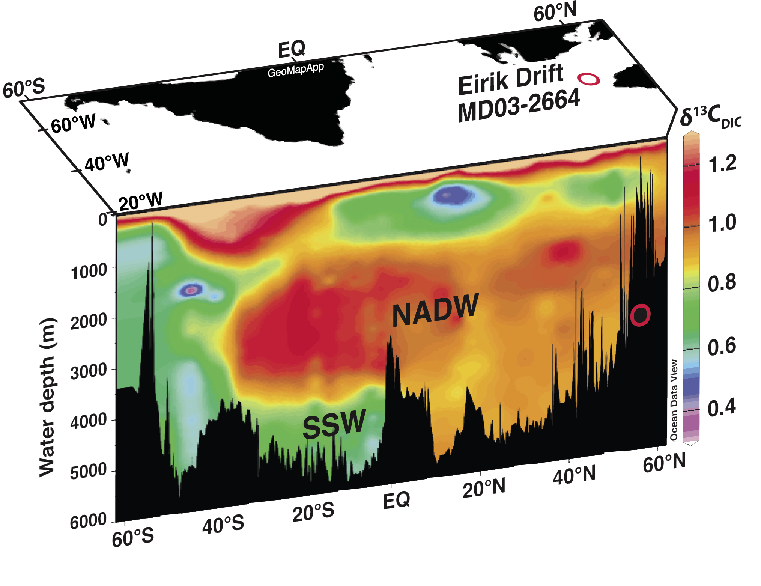
Figure 1: The location of Eirik Drift core site MD03-2664 (red circle: 57°26’N, 48°36’W; 3442 m water depth) plotted geographically and projected onto the mid-Atlantic topographic profile. Colors show the modern carbon isotopic composition of dissolved inorganic carbon (δ13CDIC; Key et al. 2004). Note the strong influence of high-δ13C North Atlantic Deep Water (NADW) in the modern Atlantic, overlying low-δ13C Southern Source Waters (SSW). Figure modified from Galaasen et al. (2014). |
Galaasen et al. (2014) reconstructed variability in NADW over the LIG using epibenthic foraminifera C. wuellerstorfi δ13C from the Eirik Drift (Fig. 1). This foraminifera records the ambient bottom water δ13C in its shell (e.g. Duplessy et al. 1984), hence it can be used to map out the distribution and circulation of water masses in the Atlantic interior (Fig. 1). The rapid sediment accumulation of ~35 cm ka-1 at Eirik Drift allowed us to reconstruct variability in newly formed Lower NADW with a high temporal resolution of ~30 years.
The Eirik Drift bottom water δ13C record indicates that NADW circulation was stable on multi-millennial timescales during the LIG, consistent with previous studies (e.g. Adkins et al. 1997). However, zooming in on shorter timescales reveals that this stable circulation state was interrupted repeatedly as the influence of NADW waned (bottom water δ13C decreased; Fig. 2) and Southern Source Water (SSW) advanced to fill the deep Atlantic. These transient NADW reductions reflect marked shifts in the circulation pattern and spatial geometry of the deep Atlantic hydrography, with shoaling of NADW and northward expansion of SSW (Fig. 1). Although difficult to determine precisely, each of these anomalies appears to have lasted several centuries before recovering, operating as if the circulation was near a threshold, but occasionally flickering back and forth across it. A critical question is then, what pushed the circulation towards this threshold and triggered these NADW reductions? Buoyancy gain in the NADW source regions likely played a key role.
 |
|
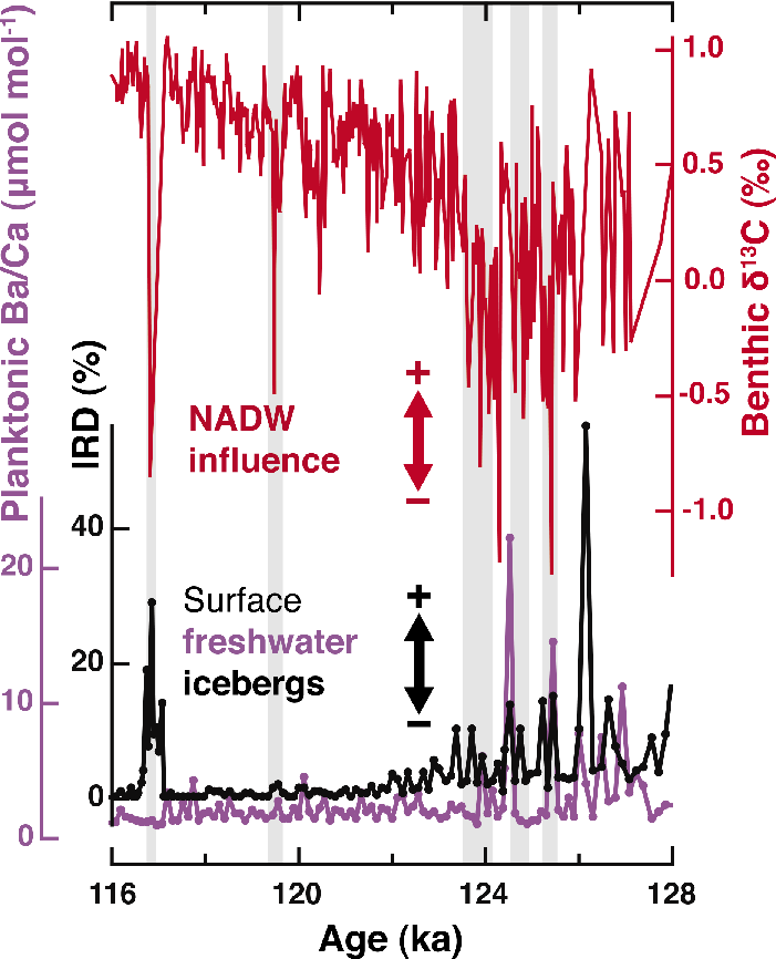
Figure 2: Eirik Drift sediment core MD03-2664 records across the LIG, focused on the Marine Isotope Stage 5e benthic δ18O plateau, (116.1-128.0 ka; Shackleton et al. 2002; Shackleton et al. 2003): Red curve: δ13C measured on shells of the epibenthic foraminifera C. wuellerstorfi; Purple curve: Ba/Ca ratio in shells of the planktonic foraminifera N. pachyderma (s); Black curve: Ice-rafted debris (IRD) percentage in the coarse fraction. Gray shading highlights intervals of reduced bottom water δ13C and NADW influence. Figure modified from Galaasen et al. (2014). |
The transient NADW perturbations were more pronounced and more frequent around the early part of the LIG interval. This period was characterized by peak Northern Hemisphere warmth (Otto-Bliesner et al. 2006; NEEM community members 2013) and high input of icebergs (ice-rafted debris (IRD) increases) and freshwater (N. pachyderma (s) Ba/Ca increases) at the sea surface in the Eirik Drift region (Fig. 2). The last and most prominent of the NADW anomalies during the early LIG (at ~124 ka) was also associated with an outburst flood analogous to the one believed to have triggered the 8.2 ka event, when large amounts of freshwater entered the North Atlantic through the Labrador Sea (Nicholl et al. 2012; Galaasen et al. 2014). Taken together, this highlights buoyancy gain from a generally warm background climate and episodic freshwater inputs as the trigger for the transient NADW anomalies of the LIG. Increases in the abundances of N. pachyderma (s) in the Eirik Drift core also indicate that each of the NADW anomalies was associated with an increased influence of polar, i.e. cold and fresh surface water (see Galaasen et al. 2014). A similar pattern of repeating and transient polar water expansions during the LIG was also found in the northeastern North Atlantic (Mokeddem et al. 2014). This suggests that the hydrographic surface water anomalies detected at the Eirik drift site might in fact have extended across the subpolar North Atlantic, indicating a strong coupling between surface and deep ocean conditions.
Interglacial NADW instability
Previous studies have suggested that NADW ventilation was generally suppressed during the early part of the LIG (e.g. Sánchez Goñi et al. 2012). The new high-resolution Eirik Drift record revises this notion, suggesting rather that several centennial-scale NADW changes occurred superimposed on a longer-term stable circulation state that was established at the start of the LIG benthic δ18O plateau (e.g. Adkins et al. 1997). However, the dimension of these NADW reductions remains unclear. While apparent in the deepest parts of the northeast (Hodell et al. 2009) and northwest Atlantic (Galaasen et al. 2014), suggesting NADW shoaled, determining how far will require additional constraints from shallower water depths.
High-resolution records of NADW variability are now available for both the Holocene and LIG, providing new insights into the stability of NADW under warm climate conditions. In both interglacials, NADW reductions cluster around the early phase. This suggests that retreating ice masses remnant from the prior glaciation were important triggers for NADW perturbations (Kleiven et al. 2008; Galaasen et al. 2014). Yet, while the Holocene experienced only one substantial perturbation to the ventilation of NADW, associated with the 8.2 ka event (Ellison et al. 2006; Kleiven et al. 2008), the LIG had several more (Fig. 2). Indeed, NADW reductions may not even have been limited to the phase of peak warmth and ice retreat during the early part of LIG. The Eirik Drift data indicate that NADW changes also occurred during the later phases of the LIG (Fig. 2).
Although these variations still need to be replicated using other high-resolution sites, the increased frequency of NADW reductions during the LIG compared to the Holocene may suggest that deep Atlantic ventilation is increasingly vulnerable as its source region warms and freshens beyond today’s levels. Further studies, including data-model comparisons and extending high-resolution records to previous interglacials, may help constrain where that potential buoyancy threshold lies and elucidate its full consequences for the circulation of the deep Atlantic.
data
The Eirik Drift core MD03-2664 epibenthic foraminifera stable isotope data are available as supplementary material to Galaasen et al. (2014).
affiliations
1Department of Earth Science and Bjerknes Centre for Climate Research, University of Bergen, Norway
2Uni Climate, Uni Research, Bergen, Norway
3Laboratoire des Sciences du Climat et de l’Environnement/IPSL, CEA/CNRS/UVSQ, Gif-sur-Yvette, France
contact
Eirik V. Galaasen: eirik.galaasengeo.uib.no
references
Adkins JF et al. (1997) Nature 390: 154-156
Duplessy JC et al. (1984) Quat Res 21: 225-243
Ellison CRW et al. (2006) Science 312: 1929-1932
Galaasen EV et al. (2014) Science 343: 1129-1132
Hodell DA et al. (2009) Earth Planet Sci Lett 288: 10-19
Key RM et al. (2004) Global Biogeochem Cycles 18, doi:10.1029/2004GB002247
Kleiven HKF et al. (2008) Science 319: 60-64
Mokeddem Z et al. (2014) PNAS 111: 11263-11268
NEEM community members (2013) Nature 493: 489-494
Nicholl JAL et al. (2012) Nat Geosci 5: 901-904
Otto-Bliesner BL et al. (2006) Science 311: 1751-1753
Sánchez Goñi MF et al. (2012) Geology 40: 627-630
Shackleton NJ et al. (2002) Quat Res 58: 14-16
Shackleton NJ et al. (2003) Global Planet Change 36: 151-155
Gianluca Marino1 and Rainer Zahn2,3
The Agulhas Leakage is a key component of the Atlantic Meridional Overturning Circulation. Unraveling the past patterns of leakage variability and associated heat and salt anomalies into the Atlantic Ocean holds clues for their role in ocean and climate changes.
The Atlantic Meridional Overturning Circulation (AMOC) modulates climate on a range of temporal and spatial scales. The northward heat transport associated with its upper limb ameliorates the North Atlantic climate, while its southward flowing lower limb transfers carbon from the atmosphere into the ocean interior (Visbeck 2007; Lozier 2012). Processes taking place in the Northern Hemisphere are historically regarded as the main drivers of the AMOC through their direct influence on the North Atlantic Deep Water (NADW) formation (Lozier 2012). Mounting evidence, however, emphasizes that the inter-ocean exchange of water south of Africa (Beal et al. 2011) and the upwelling of deep water offshore Antarctica (Visbeck 2007) are also potentially important control factors for the AMOC. We are focusing here on the transport of warm and saline waters from the subtropical Indian Ocean by the Agulhas Current, which flows southward along the shelf edge of southern Africa. While most of the Agulhas Current water recirculates into the Indian Ocean, a variable fraction, Agulhas Leakage (AL), escapes into the South Atlantic Ocean (Beal et al. 2011). Recent studies contend that the AL sets the southern control for the Atlantic upper ocean buoyancy budget and thus ultimately for the AMOC variability. Potential mechanisms for buoyancy control include planetary-wave adjustments in the Atlantic thermocline and/or advection of salt to the NADW formation sites (Beal et al. 2011 and references therein).
Paleo-reconstructions of the Agulhas Leakage
 |
|
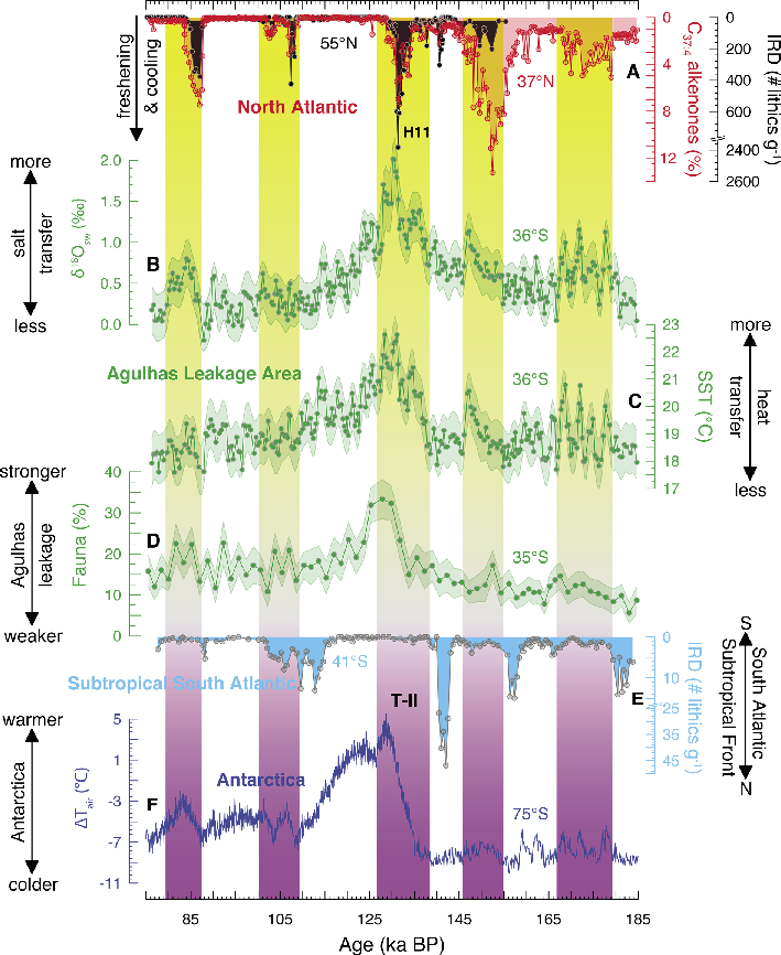
Figure 1: Agulhas leakage variability and interhemispheric climate change across the penultimate glacial-interglacial cycle. (A) North Atlantic Ice Rafted Debris (IRD, black) from ODP site 980 (Oppo et al. 2006) and tetraunsaturated alkenones (C37:4, red) from MD01-2444 (Martrat et al. 2007). (B, C) Seawater stable oxygen isotopes (δ18OSW) and sea surface temperatures (SST) from MD96-2080 (Marino et al. 2013). (D) Agulhas Leakage Fauna from GeoB3603-2 (Peeters et al. 2004). Uncertainty envelopes (2σ) are shown in B-D. (E) IRD from MD02-2588 (Marino et al. 2013). (F) Antarctic temperature anomaly from EPICA Dome C ice core (Jouzel et al. 2007). Vertical bands highlight intervals of North Atlantic cooling and Agulhas leakage strengthening. T-II=glacial Termination II; H11=Heinrich event 11. Figure modified from Marino et al. (2013). |
Several approaches have been used to investigate past AL dynamics. In their seminal study, Peeters et al. (2004) tracked the inter-ocean transport of Indian Ocean subtropical waters into the South Atlantic, using variations in tropical-subtropical planktic foraminifera, the Agulhas Leakage Fauna. From reconstructions of sea surface temperature (SST) and productivity changes Bard and Rickaby (2009) inferred the position of the Subtropical Front. Its meridional migrations reflect the oceanographic response to changes in the westerlies, impacting the width of the Indian-to-Atlantic oceanic gateway and, in turn, the inter-ocean water exchange (Beal et al. 2011). SST and seawater stable oxygen isotope (δ18Osw, a qualitative proxy for salinity) fluctuations, based on paired Mg/Ca-δ18O data in planktic foraminifera, allowed changes in inter-ocean heat and salt transports to be deciphered (Marino et al. 2013). All these reconstructions consistently show that the AL intensified during glacial terminations. However, comparison of high- (Marino et al. 2013) and low-resolution (Peeters et al, 2004) records spanning the penultimate glacial-interglacial cycle reveal that maxima in salinity, SST, and (where sufficiently resolved) faunal assemblages associated with the AL, as well as southward shifts of the regional oceanic fronts, were not limited to the prominent change across glacial Termination II (T-II). Rather smaller-scale maxima also coincided with several millennial-scale episodes of North Atlantic cooling and freshening and concurrent Antarctic warming during glacial and interglacial times (Fig. 1A-F).
Millennial-scale Agulhas Leakage variability
The paleo-evidence discussed above testifies to the link between variations in AL strength and interhemispheric or even global climate changes. In particular the Pleistocene glacial terminations feature prominent AL events. The detailed paleoceanographic reconstructions spanning T-II (Fig. 1) document that: (1) the AL maximum of T-II coincided with Heinrich event 11 (Marino et al. 2013), when the North Atlantic was cold and the AMOC weak (Fig. 1A-D); (2) as was the case during earlier glacial terminations (Peeters et al. 2004), the AL maximum was limited to the termination and did not extend into the subsequent interglacial, which featured only transient and low-amplitude AL intensifications (Marino et al. 2013) (Fig 1B-D); (3) more anticyclonic eddies carrying warm and saline waters entered the South Atlantic (Scussolini et al. 2013).
 |
|
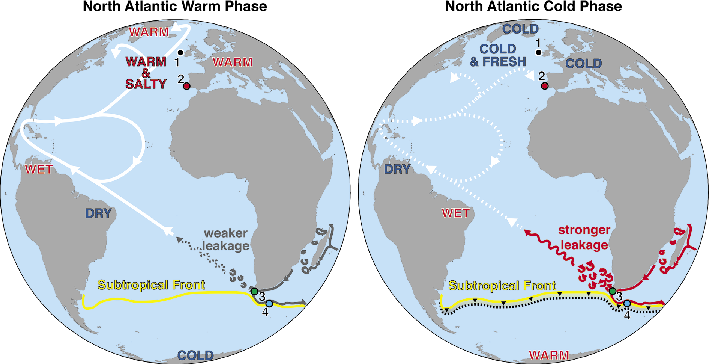
Figure 2: Sketch illustrating the relationship between Agulhas Leakage (AL) and North Atlantic climate. North Atlantic warm phase; the Atlantic Meridional Overturning Circulation (AMOC) is strong, while the AL is weak. North Atlantic cold phase; the AMOC weakens, likely due to enhanced freshwater discharge into the North Atlantic. The attendant changes in the interhemispheric ocean and atmospheric circulation cause the southward shift and potential intensification of the mid-latitude westerlies in the Southern Hemisphere, accompanied by the southward migration of the Subtropical Front that strengthens the AL. Core locations are shown: ODP 980 (1), MD01-2444 (2), MD96-2080, GeoB3603-2 (3) and MD02-2588 (4). |
Based on these observations and previous paleoceanographic analysis, we propose that the AL and its influence on the South Atlantic hydrography in the past were dominated by variability on a millennial timescale. The “terminal leakage events” during glacial-interglacial transitions were millennial-scale maxima of inter-ocean transport that, like their smaller scale counterparts, developed in response to AMOC weakening and ensuing North Atlantic cooling (Fig. 2). This initiated a sequence of feedback responses that impacted the Southern Hemisphere westerlies (Lee et al. 2011), with knock-on consequences for the position of the regional oceanic fronts and AL strength. During glacial terminations, large CO2 rise (Toggweiler et al. 2006) and sustained Southern Ocean warming (Knorr and Lohmann 2007) may explain the particularly strong AL indicated by the data, e.g. by amplifying the responses of the Southern Hemisphere westerlies and the Subtropical Front. Nevertheless, questions remain on the postulated interplay between changing wind field and the AL strength. In fact, the scenarios inferred from the paleorecords seem to disagree with state-of-the-art numerical simulations, which, however, are only run with modern boundary conditions (Durgadoo et al. 2013).
Outlook
Despite the strong paleoceanographic evidence for an AL involvement in glacial-interglacial transitions and possibly in more abrupt climate episodes (Peeters et al. 2004; Marino et al. 2013), it remains to be determined whether the AL responded passively to these changes or played an active role in them. Analysis of the temporal phasing suggests that AL maxima lead AMOC strengthening. Based on that, one can argue that the AL was both a passive and an active player. The leakage intensified passively in response to AMOC weakening/North Atlantic cooling (passive role), but the attendant negative buoyancy forcing may then have actively contributed or even caused the subsequent AMOC resumption (Knorr and Lohmann 2007; Beal et al. 2011).
Several limitations prevent us from unambiguously solving this riddle. The detailed phasing between AL fluctuations and changing AMOC is limited by difficulties inherent in aligning the paleo-records from the southern tip of Africa with those from the North Atlantic and Antarctica (Marino et al. 2013). Paleo-modeling supports the hypothesis that intensified leakage and AMOC resumption are coupled (Knorr and Lohmann 2007). Explaining the apparent temporal offset between AL strengthening and AMOC resumption would require a buoyancy threshold for reinvigorating NADW formation. However, quantitatively constraining the buoyancy threshold is limited by our ability to quantitatively translate paleo-δ18Osw variations into salinity changes, because the δ18Osw-salinity relationship varied in the past particularly in regions dominated by advective processes (Rohling and Bigg 1998).
To identify the exact role of the AL in climate change, the focus of paleoceanographic research must shift to a quantitative analysis of the heat and salt transports around the southern tip of Africa and across the Atlantic Ocean. The high-amplitude leakage events at glacial terminations may be used to reconstruct with a higher degree of confidence the signal propagation into and across the Atlantic Ocean, thereby serving as templates for the millennial-scale leakage maxima that punctuated glacial and interglacial climates.
acknowledgements
This research was funded by European Commission Seventh Framework Programme, projects “Past4Future” (grant no. 243908) and “Gateways” (grant no. 238512). G. Marino also thanks the Universitat Autonoma de Barcelona (postdoctoral research grant no. PS-688-01/08) and the Spanish Ministry of Science and Innovation (PROCARSO project, grant no. CGL2009-10806).
data
Data presented here are available from the corresponding author and are in the process of being submitted to NOAA NCDC.
affiliations
1Research School of Earth Sciences, The Australian National University, Canberra, Australia
2Institució Catalana de Recerca i Estudis Avançats (ICREA), Barcelona, Spain
3Institut de Ciència i Tecnologia Ambientals (ICTA) and Departament de Física, Universitat Autònoma de Barcelona, Cerdanyola del Vallès, Spain
contact
Gianluca Marino: gianluca.marinoanu.edu.au
references
Bard E, Rickaby REM (2009) Nature 460: 380-393
Beal LM et al. (2011) Nature 472: 429-436
Durgadoo JV et al. (2013) J Phys Oceanogr 43: 2113-2131
Jouzel J et al. (2007) Science 317: 793-796
Knorr G, Lohmann G (2007) Geochem Geophys Geosyst 8, doi:10.1029/2007GC001604
Lee S-Y et al. (2011) Paleoceanography 26, doi:10.1029/2010PA002004
Lozier MS (2012) Annu Rev Mar Sci 4: 291-315
Marino G et al. (2013) Paleoceanography 28: 599-606
Martrat B et al. (2007) Science 317: 502-507
Oppo DW et al. (2006) Quat Sci Rev 25: 3268-3277
Peeters FJC et al. (2004) Nature 430: 661-665
Rohling EJ, Bigg GR (1998) J Geophys Res Oceans 103: 1307-1318
Scussolini P et al. (2013) Clim Past 9: 2631-2639
Toggweiler JR et al. (2006) Paleoceanography 21, doi:10.1029/2005PA001154
Longbin Sha1, H. Jiang1, M-S. Seidenkrantz2, K.L. Knudsen2, J. Olsen3 and A. Kuijpers4
A diatom-based sea-ice transfer function was developed for the north-western Atlantic. A first reconstruction of sea-ice concentration off West Greenland shows multi-centennial oscillations superimposed an overall trend of expanding sea ice over the last 5000 years.
Sea ice is a sensitive component of the Earth’s climate system. It acts as an effective insulator between the oceans and the atmosphere, restricting the exchange of heat, mass, momentum and chemical constituents (Divine and Dick 2006). However, reliable and continuous observations of sea ice only exist since 1978. Extending the sea-ice record further back in time is necessary, e.g. to provide well-constrained boundary conditions and benchmarks for model simulations.
 |
|
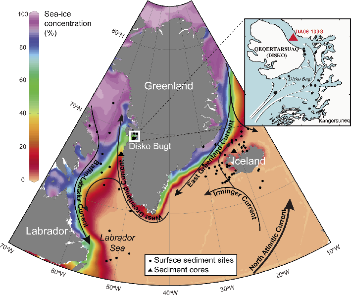
Figure 1: Maps of the NW Atlantic, indicating the prevailing surface currents, the distribution of surface sediment samples for the regional diatom-based sea-ice transfer function, and the locations of the sediment cores mentioned in the text. The satellite April sea-ice concentration for 1979-2010 is indicated as a background. |
Diatoms are marine siliceous algae which have been used successfully for quantitative reconstructions of sea-ice conditions, mostly in the Southern Ocean (Crosta et al. 1998; Gersonde et al. 2005) but also in the north-western Atlantic (Justwan and Koç Karpuz 2008). We have now established a new diatom-based transfer function for past sea-ice concentrations (SIC) for the region off West Greenland (Fig. 1) and applied it to produce a ca. 5000 year-long reconstruction (Sha et al. 2014).
Modern diatom-SIC dataset
 |
|
Figure 2: Sea-ice records over the last century and the last 5000 years, respectively. (A) From bottom to top: Reconstructed SIC (blue) from core GA306-BC4 compared with the SIC from satellite observation (red) and model output (purple), and annual mean instrumental temperatures (orange). Original data are shown as thin lines; thick lines are 7-point weighted moving averages. (B) From bottom to top: Reconstructed SIC (blue) and warm-water diatom taxa (green) from core DA06-139G, reconstructed May SIC from core MD99-2269 (purple; Justwan and Koç Karpuz 2008). The gray shading indicates value below each record’s mean. Approximate time intervals for historical NE Atlantic climate events are given (LIA: Little Ice Age; MCA: Medieval Climate Anomaly; DACP: Dark Ages Cold Period; RWP: Roman Warm Period; HTM: Holocene Thermal Maximum). Figure modified from Sha et al. (2014). |
We determine the modern calibration between diatom assemblages and SIC data based on (1) diatom assemblage analysis from 72 surface sediment samples from the north-western Atlantic (Fig. 1) and (2) monthly means of the satellite SIC data collected from Nimbus-7 SMMR and DMSP SSM/I-SSMIS Passive Microwave Data.
Diatom assemblages are distinguished, with respect to monthly average SIC, using canonical coordination techniques (ter Braak and Šmilauer 2002; Lepš and Šmilauer 2003). Of the 12 monthly mean SICs, only April, August, October, and November SICs influence variations in the diatom data noticeably. And of those months, forward selection and an associated Monte Carlo permutation test reveal that only April and August SICs explained a statistically significant (p ≤0.001) amount of variation in the diatom assemblage data, representing 52% of the total canonical variance. The April SIC alone accounts for 38% (August 14%), suggesting that it is the most important environmental control on diatom ecology in this area. This is coherent with the observation that April is one of the most critical months for diatom blooms as the combined light and temperature conditions are often optimal in this month.
Transfer function for April SIC
Multiple numerical reconstruction methods such as Modern Analogue Technique (MAT, based on one to five analogues), Weight Averaging regression (WA), and Weighted Averaging with Partial Least Squares regression (WA-PLS, based on one to five components) were tested and evaluated for developing the most reliable diatom-based transfer function for April SIC. These tests reveal that the numerical reconstruction based on WA-PLS with three components results in the most reliable diatom-based SIC for the area (see Sha et al. 2014 for details).
Testing the SIC reconstruction
In order to test the reliability of the diatom-based SIC reconstruction as a measure for paleoceanographic changes in the north-western Atlantic region, we compared the reconstructed SIC of the last ~75 years from box core GA306-BC4 (445 m water depth) with the satellite SIC record for 1979-2006 (Fig. 2A). Additionally, we compared our reconstructed SIC with the model SIC from the HasISST 1.1 dataset (Rayner et al. 2003) during 1953−2006, and with the mean water temperature in the upper 200 m west of Fylla Bank during 1963-2006.
The diatom-based reconstructed SIC exhibits a generally similar distribution pattern to the satellite and model sea-ice data, as well as the instrumental temperature records, although with a few temporal differences (Fig. 2A). These temporal differences may be caused by uncertainties in the chronology and the low temporal resolution of the sediment core. However, the comparison suggests that overall our diatom-based SIC transfer function is a reliable method for studying paleoceanographic changes in the north-western Atlantic.
A 5000-year record of April SIC
The transfer function was applied to the diatom assemblages from core DA06-139G (384 m water depth, Fig. 1) to establish an April SIC record for the last 5000 years in the Disko Bugt (Fig. 2B; Sha et al. 2014). The reconstructed SIC values varied between 25-95% around a mean of 55%, with an overall trend towards increasing sea ice. Between 5000 and 3860 cal yr BP, our results suggest that the SIC was generally below the mean value except for a short period around 4900 cal yr BP. This coincides with relatively warm conditions suggested by an abundance of warm-water diatom species (Fig. 2B). This period corresponds to the latest part of the Holocene Thermal Maximum. Between 3860 and 1510 cal yr BP SIC oscillated around the mean value. From 1510-1120 cal yr BP and after 650 cal yr BP was above the mean, indicating that sea-ice cover in Disko Bugt was particularly extensive.
Warm-water diatom species reflect warm Atlantic water, as evidenced by the abundant distributions in surface sediments (Sha et al. 2014). The distribution pattern of sea-ice diatom species correlates well with the strength of cold polar water from the East Greenland Current (Sha et al. 2014). Agreement between reconstructed SIC and changes in the diatom species suggests that sea-ice conditions in Disko Bugt were influenced by variations in the relative strength of the two main components of the West Greenland Current, i.e. the cold East Greenland Current carrying polar water from the Arctic Ocean and the relatively warm Irminger Current of Atlantic origin (Fig. 2B). The North Icelandic shelf was influenced by both the Irminger Current and the East Greenland Current. A diatom-inferred May SIC record from there, shows a similar SIC pattern to that found in the Disko Bugt, particularly during the time periods before 3500 cal yr BP and after 2000 cal yr BP (Justwan and Koç Karpuz 2008; Fig. 2B). Differences observed between the two reconstructions during the 3500-2000 cal yr BP time interval may reflect that the different approaches used to reconstruct past sea-ice variations could describe different aspects of sea-ice cover. Finally, a preliminary comparison between the reconstructed SIC record and total solar irradiance suggests a relationship between solar forcing and sea-ice changes (Sha et al. 2014).
Outlook
We established a new diatom-based SIC transfer function for the north-western Atlantic region and provided a quantitative reconstruction of April sea-ice conditions in this region over the last 5000 years. Discussions remain about what causes sea-ice variations in the area and more detailed analysis are currently being performed to decipher the controlling factors.
In spite of its advantage for quantitatively extending sea-ice record to geological past, our diatom-based SIC transfer function still has some limitation due to re-suspension and preservation of some diatom species through time. In order to reconstruct sea-ice variability with confidence, a multi-method strategy will be focused on, which may capture complementary information from the complex relationships between surface sediment diatoms and the modern environmental variables.
affiliations
1Key Laboratory of Geographic Information Science, East China Normal University, Shanghai, China
2Centre for Past Climate Studies and Arctic Research Centre, Aarhus University, Denmark
3Department of Physics and Astronomy, Aarhus University, Denmark
4Geological Survey of Denmark and Greenland (GEUS), Copenhagen, Denmark
contact
Longbin Sha: shalongbinhotmail.com
references
Crosta X et al. (1998) Paleoceanography 13: 284-297
Divine DV, Dick C (2006) J Geophys Res 111, doi:10.1029/2004JC002851
Gersonde R et al. (2005) Quat Sci Rev 24: 869-896
Justwan A, Koç Karpuz N (2008) Mar Micropaleontol 66: 264-278
Rayner NA et al. (2003) J Geophys Res Atmos 108, doi:10.1029/2002JD002670
Sha L et al. (2014) Palaeogeog Palaeoclimatol Palaeoecol 403: 66-79
Dorthe Dahl-Jensen
Climate change is not only of concern to scientists but also to the public, media, and policymakers. Therefore, it is critical that EU projects dedicate effort to reaching out to these groups. This article describes the approaches taken by Past4Future.
 |
|
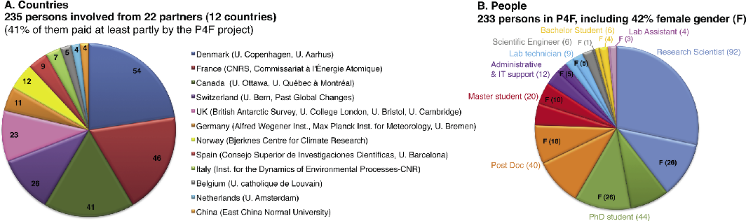
Figure 1: Statistics related to the structure of the Past4Future project, including (A) the project partners and their national affiliations and (B) the functions and gender of people involved. |
 |
|
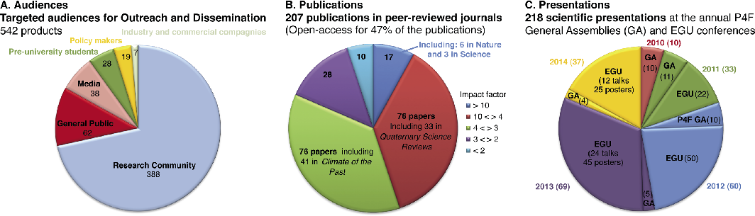
Figure 2: Statistics related to the products of the Past4Future project, including (A) its target audiences, (B) scientific publications and (C) presentations (as of mid-November 2014). |
The Past4Future project was a five-year project combining the expertise of 22 European and associated international project partners (Fig. 1). The project’s core objective was to inform our knowledge about future climate and possible abrupt changes by researching similar conditions in the past and share the findings widely. Therefore, a substantial part of efforts and resources went into communicating the project results to a broad audience, including scientists both within and external to the climate science community, as well as policymakers and the public (Fig. 2A). This article provides an overview of the efforts undertaken and describes some of the achievements and barriers encountered along the way.
Communicating with stakeholders
Early in the project, a stakeholder survey was carried out to identify the method of dissemination that would be of most value to the main user groups, including scientists, policymakers, and the public. While the survey confirmed a general demand for scientific information, demands also extended to the clarity of communication. Scientific issues need to be presented in a clear way, which includes that robust results are identified and distinguished from more speculative scenarios and unlikely developments. Due to the complexity of the scientific issues involved in climate change, many misconceptions and contradictory statements appear to exist, particularly among the public.
Getting feedback from the stakeholders turned out to be a major difficulty. Accordingly, we only received complete information from 13 of the 141 contacted (Thing 2013). This might illustrate that stakeholders are busy people and that a science survey has a low priority for them. Communication must therefore be particularly targeted and brief.
From the feedback we had received, it become very clear that stakeholders do not want information to be presented in the form of glossy brochures, and that information using the Intergovernmental Panel on Climate Change (IPCC) way of communicating uncertainty in text and graphs is preferred. Stakeholders preferred that shorter timescales of climate change impacts (10-100 years, within human lifetimes) were reported, although longer timescales were also acknowledged to be relevant. Information on most aspects of the climate system was considered important, with temperature and sea level considered top priorities.
Based on the feedback from the survey, we focused Past4Future communication efforts on participation in and contribution to the Fifth Assessment Report of IPCC’s Working Group 1 (IPCC 2013), on press material related to publications by Past4Future researchers, and on press sessions at the EGU meetings in 2013 and 2014. Furthermore, final Past4Future findings were presented in three summary papers during a lunch meeting for decision makers in Brussels.
Communicating results to the scientific community
The scientific communication in Past4Future focused on peer-reviewed publications. A total of 207 papers in peer-reviewed journals, 97 of them open access, have acknowledged the Past4Future grant from the EU’s Seventh Framework Programme (Fig. 2B, and full list at www.past4future.eu). These papers have been cited at least 777 times (as of Nov 2014), resulting in an overall h-index of 13.
The publications present major results on the behavior of the climate system in the last and the present interglacial periods. The systematic study of changes in these periods in the framework of Past4Future allows us to improve our understanding of the causes and risks of abrupt changes by aligning the timescales of paleoclimate records and using transient model simulations. And in line with one of the key project ambitions, a significant number of the papers were cited in the Fifth Assessment Report of the Working Group 1 of the IPCC.
In each of the five years of the project, Past4Future scientists planned and organized a session at the general assembly of the European Geosciences Union (EGU) where ongoing research and major results were communicated through oral presentations, traditional posters, and in the new format of interactive two-minute presentations. The sessions were among the biggest and most attended in the climate section of EGU, featuring between 22 and 69 presentations and attracting hundreds of attendees each year (Fig. 2C).
Global visibility of Past4Future was increased through the involvement of the global organization PAGES. Two special sections of the PAGES magazine (including the one at hand) were dedicated to Past4Future. They highlight key project results in an accessible format. The global distribution of the magazine and the project website, also hosted by PAGES, generated international synergies and brought the goals and outcomes of Past4Future to the attention of the paleoscience and wider scientific community well beyond Europe.
Data compilation and provision
As one of the dissemination and integration goals, Past4Future has produced a database of paleodata from a range of proxy archives available for the last two interglacial periods. In 2012, it was decided to use the PANGAEA database for the proxy records so they would be available for the entire scientific community. At present, 457 datasets directly related to Past4Future are in the database at www.pangaea.de. In addition to the proxy metadatabase, a modeling database has been created on the www.past4future.eu website as a portal for the project’s model output.
Providing open access to Past4Future products was a key goal that was very successfully met, providing a valuable platform for ongoing research. Leveraging and building communication and archival resources using the structures of PAGES and PANGAEA also ensures that the information produced by Past4Future will exist and remain accessible after the project has come to an end.
The data compilation was complemented by a review of the dating methods of paleoclimatic archives and the alignment strategies of paleoclimatic records, with the goal of producing a protocol that enabled us to correctly and consistently compare paleoclimatic records from different archive types and between remote regions. As a result, a dating and synchronization guideline report was delivered in 2012, presented in the form of a PAGES magazine article (Capron et al. 2013) and prepared for submission to Quaternary Science Reviews (Govin et al. in prep). These guidelines have been used throughout the project.
Internal project communication
Past4Future brought together an interdisciplinary team of skilled experts to advance the under-standing of interglacial climate from global paleorecords. Among the 22 partner institutions of Past4Future, 197 scientists were directly involved in the project. Amongst them, 110 (i.e. 56%) were early-career scientists, including 40 PhD students (Fig. 1D). Of these, 19 were directly funded through the Past4Future grant, the others were funded mainly through national grants that linked to the Past4Future project.
Note also that the project has a gender ratio of 42% women (Fig. 1D). This is very high for paleoclimate science which has traditionally been dominated by male researchers.
Encouraging young researchers to be mobile and to expand their network was an important goal for Past4Future. To facilitate educational benefit for students in the project we maintained a roster of relevant laboratory and field courses available for PhD and MSc students. This meant that Past4Future’s researchers-in-training could choose to attend courses offered in other institutes from other nations.
A General Assembly for project participants was organized in each year of the project (Fig. 2B), during which the team could meet and exchange information about their latest results and plan and coordinate activities. Besides reports and presentations by the working groups, we organized special sessions for young scientists and a discussion session with decision makers, in which the EU Commissioner for Climate Action, Connie Hedegaard, participated.
Outlook
A final goal of the project is the dissemination of products targeting decision makers. To this end, a lunch meeting is held in Brussels where the major results generated by Past4Future are presented to policy and decision makers. Through an integrative approach combining information from climate model simulations and paleoclimate records, Past4Future reached far and accomplished a lot in understanding the processes that controlled the climate during the last two interglacial periods. The results have been published and presented at big meeting as the EGU. In addition the results have influenced the IPCC Fifth Assessment Report. I am pleased to conclude that Past4Future has lived up to its vision and fulfilled its mission to play an important role in applying knowledge of the past for the benefit of our common future.
affiliation
Centre for Ice and Climate, Niels Bohr Institute, University of Copenhagen, Denmark
Coordinator of Past4Future.
contact
Dorthe Dahl-Jensen: ddjnbi.ku.dk
references
Shaun A. Marcott1 and Jeremy D. Shakun2
Mount Hood, USA, 13-16 October 2014
 |
|
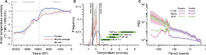
Figure 1: (A) Global mean temperature from proxies (Marcott et al. 2013; Shakun et al. 2012) and models (Liu et al. 2014). (B) Histograms of the Holocene time series in (A) showing how the distribution of Holocene temperatures compare to the 20th century instrumental range and IPCC projections for 2100 (Collins et al. 2014). (C) Power Spectral Density (PSD) of sea surface temperature variance for Holocene time series (Laepple and Huybers 2014). RCP = Representative Concentration Pathway. |
The Holocene, which covers the last 11,700 years including the entire time span of human civilization, stands out as an interval of relative climate stability. A major goal of the paleoclimate community has been to develop a longer-term perspective on climate change to understand natural variability and provide context for future warming, which model projections indicate will substantially exceed even the warmest Holocene conditions (Fig. 1b). Major efforts by PAGES working groups to synthesize and analyze global paleoclimate records and model simulations of the late Quaternary have mostly focused on the Common Era of the past two millennia (PAGES 2k), the last deglaciation (SynTraCE-21), and past interglacials (PIGS), with relatively less attention paid to the transient evolution of the Holocene. Given that the Holocene is the closest analog for today’s climate state and covered by abundant proxy data, coordinated scrutiny of the Earth System over this timeframe should add important information regarding future climate change.
To better define both the short and long-term goals of the scientific community working on reconstructing and modeling Holocene climate, a meeting was held at Timberline Lodge at Mount Hood, Oregon. The meeting focused primarily on three themes: regional and global climate trends, variability in space and time, and data-model comparison.
Trends
As highlighted in Marcott et al. (2013) and Liu et al. (2014), a data-model disparity exists for global surface temperature during the Holocene that is not apparent for the last deglaciation, with proxies recording a long-term cooling and models simulating a warming (Fig. 1a). This “conundrum” was distilled to either relating to seasonal biases in the data, incomplete forcings, or insufficiently sensitive feedbacks in the models, or a combination of these. Seasonal biases in paleoclimate proxies pose a major challenge for reconstructing annual temperatures and comparing unlike datasets (e.g. Mix 2006), particularly during the Holocene when seasonal insolation changes were strong compared to other forcings that act across the year. Model simulations are likewise challenged by initiating glacial inceptions from insolation forcing and are limited by some weakly constrained forcing inputs, such as volcanic and solar activity. Resolving the Holocene temperature conundrum is important for understanding the forcing-response mechanisms during the current interglacial and for putting present and future climate into context, as the global temperature trend dictates to what extent today’s earth system has already exited the Holocene range (Fig. 1b).
Variability
Temperature, precipitation, and glacier variability at sub-millennial frequencies and in multiple regions was also discussed. Given the relatively small changes in climate during the Holocene, differentiating a meaningful climate signal from proxy or local noise was highlighted as a critical goal for accurately reconstructing Holocene variability. This issue is central to comparisons between data and model results, which currently disagree over the spectrum of regional variability. Models tend to suppress the regional-scale variability seen by proxies at multi-decadal and longer periods (Fig. 1c). This discrepancy suggests that models may not generate enough low frequency internal variability, thus limiting their ability to produce accurate simulations of climate at longer time scales (Laepple and Huybers 2014).
Proposing a PAGES Working Group
To move forward, a PAGES Holocene working group was agreed to be a useful bridge between the existing PAGES 2k project and previous efforts focusing on the deglaciation. The focus should be on both temperature and hydroclimate changes across the Holocene, and include independent modeling and data analysis efforts. Forward modeling will be an important link between the modeling and proxy communities that will enable true data-model comparisons. The initial phase of the working group should focus on developing a Holocene database, first synthesizing existing compilations, and then incorporating remaining data. Community involvement and potential crowd sourcing should be encouraged to finalize the database and maximize its analysis, leading to a series of synthesis products. To run and maintain such an effort requires that dedicated personnel be supported. This could include a well-versed postdoc(s) who would lead the initial phase of the project and help steer the early scientific objectives.
acknowledgements
The meeting was sponsored by the US National Science Foundation (#1449148) and PAGES. We thank T. Kiefer, T. Laepple, Z. Liu, H. Wanner and J. Zhu for assistance.
affiliations
1Department of Geoscience, University of Wisconsin-Madison, USA
2Department of Earth and Environmental Sciences, Boston College, USA
contact
Shaun A. Marcott: smarcottwisc.edu
references
Laepple T, Huybers P (2014) PNAS 111: 16682–16687
Liu et al. (2014) PNAS: E3501–E3505
Marcott et al. (2013) Science 339: 1198-1201
Mix AC (2006) Quat Sci Rev 25: 1147–1149
Antoni Rosell-Melé1, E.L. McClymont2, P.S. Dekens3, H. Dowsett4, A.M. Haywood5 and C. Pelejero6
Barcelona, Catalonia, Spain, 17-19 September 2014
 |
|
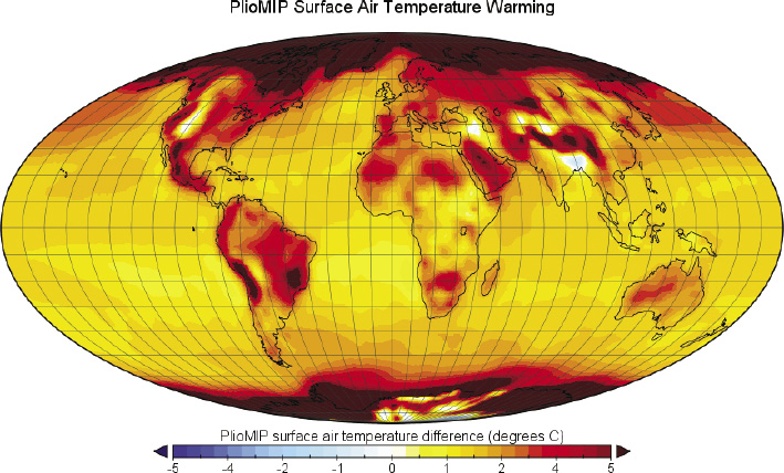
Figure 1: Mean annual surface air temperature anomaly (mid-Pliocene minus pre-industrial simulations) based on a multi-model means ensemble obtained by the Pliocene Model Intercomparison Project. Adapted from Haywood et al. (2013). |
The Pliocene epoch has often been proposed as a climate analogue for future conditions on Earth. However, despite relatively small differences in climate control factors, including atmospheric CO2 concentration, the Pliocene climate was markedly different from the modern climate. This has made the Pliocene a relevant target for validating climate models. This in turn requires confidence in the paleoclimate estimates to be able to fully ascertain model strengths and weaknesses. In this context, and in order to further develop efforts by earlier projects such as PRISM (Pliocene Research, Interpretation and Synoptic Mapping group) and PlioMIP (Pliocene Model Intercomparison Project), about 65 specialists of the international community of Pliocene researchers met at a workshop in Barcelona. The key mission was to establish guidelines to facilitate further a community wide international effort to reconstruct key climatic parameters (temperature, CO2, continental and sea ice, sea level, vegetation) in selected time intervals within the Pliocene epoch. The ultimate goal of this community effort is to provide a comprehensive global representation of Pliocene climate, which would facilitate data modeling comparisons. To this end, the workshop consisted of invited plenary talks that synthesized the current state of the art, followed by working group discussions of research priorities, and reporting and synthesis presentations towards the end of the workshop. Participants presented their current research in poster sessions.
Plenary talks highlighted the challenges of trying to reconstruct Pliocene climate and the need to reassess some concepts. These included the recognition that the Pliocene does not fit the paradigm of a “stable climate”, nor should it be considered an isolated time period, but instead part of a climate continuum, preceded by the much warmer Miocene. Thus, no specific time slice within the Pliocene will be representative of the epoch’s entire range of climate variability, while the character of Pliocene interglacials could be as variable as those of the Quaternary. Integrating or comparing models and data requires dealing with reconstructions with very different constraints on the time (e.g. series or slices with no time lapse) and spatial domains (e.g. global vs regional), all with their own uncertainties. Among the many implicit challenges, urgency was placed on the need to revise the existing Pliocene marine isotope reference templates on which time series age models are based, and the quantification of uncertainty in proxy reconstructions.
From the discussions, a consensus emerged on setting research priorities for different time lines. For instance, in the short-term, there is a need to focus efforts on the reconstruction of isotopic stages M2 through to KM3 (i.e. ca. 3.2-3.3 Ma) and on the improvement of the spatial and temporal reconstructions of proxy data sets to constrain meridional temperature gradients and conditions in high latitude environments.
In the mid-term, one of the priorities is to further the development and application of proxies and models, for instance related to precipitation, or the disentanglement of multiple environmental effects affecting our proxies of temperature and sea-level. It is also paramount to target key regions and issues on which information is lacking, such as the reconstruction of sea-ice or continental precipitation.
In the long term, efforts should focus on creating syntheses that include both relative changes (e.g. information on forcings) and absolute changes required for quantitative data-model integration, for time periods that include the early Pliocene and eventually provide space and time transect information. The priorities will be available in a more elaborate form on the workshop web site: http://jornades.uab.cat/plioclim/.
The next step of the initiative is to seek its consolidation through the creation of a formal working group, and summarize some of the discussion in research papers. We also aim to create a database to summarize the proxy data and make them accessible for further research such as data-model comparisons. The group agreed to review and reassess its objectives in a meeting in two years, to be held in Norway.
acknowledgements
The organizers thank PAGES, ICREA, EGU, and SCAR-PAIS for their financial support, ICTA-UAB for administrative support, and ICM-CSIC for allowing the use of their facilities for the workshop.
affiliations
1ICREA and Institute of Environmental Science and Technology, Universitat Autònoma de Barcelona, Catalonia, Spain
2Department of Geography, Durham University, UK
3Department of Earth & Climate Sciences, San Francisco State University, USA
4Eastern Geology & Paleoclimate Science Center, US Geological Service, Reston, USA
5School of Earth and Environment, University of Leeds, UK
6ICREA and Institut de Ciències del Mar, CSIC, Barcelona, Catalonia, Spain
contact
Antoni Rosell-Melé: antoni.roselluab.cat
reference
Andreas Schmittner1, S.L. Jaccard2, A.C. Mix1 and E.L. Sikes3
Inaugural OC3 Workshop, Bern, Switzerland, 1-3 October 2014
The stable isotopes of carbon (δ13C) provide a uniquely valuable tracer of the carbon cycle, and are an essential component for understanding changes in the Earth’s various carbon reservoirs and their relation to climate change. Its spatial distribution in the ocean is affected by circulation and fractionation during gas exchange, and carbon cycling. Foraminifera, which are microscopically small animals living near the surface (planktic) or in/on the sea floor (benthic species), incorporate the dissolved inorganic carbon (DIC) isotopic signature of the water δ13CDIC into their calcium carbonate shells, which are eventually preserved in the sediments providing a glimpse into past δ13CDIC levels. Ever since the first comparison of foraminifera δ13C data from core-top sediments with water column measurements (Duplessy et al. 1984), paleoceanographers have used foraminifera δ13C as a proxy to reconstruct past changes in ocean circulation and other environmental variables. The record is more complex than originally assumed, however, and to advance understanding requires careful consideration of these complicating factors.
The goal of the new PAGES “Ocean Circulation and Carbon Cycling” working group OC3 (http://pastglobalchanges.org/ini/wg/oc3/intro) is to synthesize sedimentary δ13C data in order to reconstruct changes in ocean circulation and carbon cycling over the last deglaciation. This time period is of particular interest since it was characterized by overall global warming and large changes in the climate system and the carbon cycle. In addition there exist well-constrained paleo-records at high temporal resolution, with a reasonable spatial distribution.
The kick-off OC3 meeting was held back-to-back with the related International Quaternary Association’s International Focus Group IPODS (Investigating Past Ocean Dynamics) in order to exploit existing connections and foster collaboration between both working groups. IPODS has similar goals of understanding deglacial circulation changes but focuses on different proxies, such as radiocarbon, and other dynamic proxies of ocean circulation (εNd, Pa/Th). Here we only report on the OC3 part of the workshop. The IPODS report is available elsewhere (Skinner and Schmittner 2014).
OC3 presentations included new efforts to simulate δ13C in comprehensive Earth System Models, simulations of deglacial changes using intermediate complexity models, and inverse modeling of the modern- and Last Glacial Maximum (LGM, 23-19 ka BP) ocean. Compilations of available data as well as new downcore records of δ13C from the Atlantic and the Pacific oceans showed coherent changes consistent with the interpretation that the deep ocean circulation changed particularly strongly in the Atlantic and at mid depths during the Heinrich Stadial 1 (HS1, 19-15 ka BP), whereas deeper layers in the South Atlantic and South Pacific changed later during the Bølling-Allerød (15-13 ka BP) coeval with the Antarctic Cold Reversal and the Younger-Dryas (13-12 ka BP).
One session explored uncertainties of δ13C reconstructions. Carbonate ion concentrations have been shown to lead to species-specific offsets between planktonic foraminifera δ13C and the water column δ13C (Spero et al. 1997).
 |
|
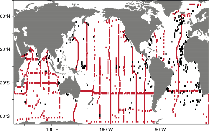
Figure 1: Map of available foraminifera δ13C data (on a 1° grid) from core-top sediment foraminifera (black; Pederson et al. 2014 plus unpublished data from A. Mix) and water column δ13CDIC(red) measurements. These two datasets will be used for calibrations. |
One of the immediate goals of OC3 is to update the original global calibration against seawater δ13C of benthic foraminiferal δ13C of Duplessy et al. (1984) by using a much larger database of both water column and core-top sediment data. Figure 1 shows the current distribution of both datasets. Preliminary analysis of these data indicates that the carbonate ion effect is also present in the benthic foraminifera δ13C data.
Discussions during breakout groups and within the plenary focused on details of data synthesis such as metadata needed, formats, and conventions for archiving individual data sets, and retrieval methods. Finally, a strategy and plan for the next steps was developed that cuts out the work until the next meeting, which will presumably be he held in 2015.
affiliations
1College of Earth, Ocean, and Atmospheric Sciences, Oregon State University, Corvallis, USA
2Institute of Geological Sciences, University of Bern, Switzerland
3Institute of Marine and Coastal Sciences, Rutgers University, New Brunswick, USA
contact
Andreas Schmittner: aschmittcoas.oregonstate.edu
references
Duplessy J-C et al. (1984) Quat Res 21: 225-243
Peterson CD et al. (2014) Paleoceanography 29: 549-563
Schmittner A et al. (2013) Biogeosciences 10: 5793-5816
Felicity Williams1, N. Hallmann2 and A. Carlson3
PALSEA2 Workshop, Lochinver, Scotland, UK, 16-22 September 2014
 |
|
Figure 1: The systematic conversion of observation into data is a cornerstone of scientific method as suggested by the marine-terminating ice margin of Nigerdlikasik Bræ in southern Greenland. Image credit: A Carlson and F Williams. |
PALSEA2 is the second phase of work to reduce the uncertainty around past ice-sheet and sea-level variability that began with the PALSEA (PALeo constraints on SEA level rise) working group co-sponsored by PAGES and INQUA. The second meeting of PALSEA2 took place against the backdrop of northwestern Scotland’s postglacial landscape. Twenty-nine people from seven countries attended to explore, discuss, and debate the methods by which large databases of past sea level and ice-sheet extent can be developed over a range of spatial and temporal scales, from the Pliocene climatic optimum to the current interglacial period. Delegates presented on the production and analysis of composite datasets, and enjoyed extensive field discussions at sites that had contributed to present day knowledge of the British and Irish ice sheets at the Last Glacial Maximum.
Cutting edge advances at the ice-sheet scale are only possible through the compilation of large datasets, highlighting the value databases offer to the scientific community. The contribution of region-specific databases to our current understanding of the Antarctic, British and Irish, and Greenland ice sheets were explored by Peter Clark, Sarah Bradley and Anders Carlson (Carlson et al. 2014; Kuchar et al. 2012; Lecavalier et al. 2014).
Discussions throughout this workshop highlighted the need for data management plans with a global scope, and the consistent and comprehensive treatment of data. Key points of agreement included the necessity of mandating the inclusion of meta-data in order to facilitate the use of sample data across multiple scientific disciplines and that the template should attempt to future-proof data to meet the demands of future analyses. The finalised protocol should also ensure the continuation of valuable conversations between the primary producers and users of the data and subsequent researchers.
Complementary approaches to structuring databases were presented. André Düsterhus outlined a thematic structure comprising the value, measures of uncertainty, associated expert knowledge, and commentary, whilst Marc Hijma presented an existing and highly detailed protocol for a post glacial database of sea level indicators (Hijma et al. in press).
Bridging the gap between geological and instrumental records, the Late Holocene is a prime target for reconstructing regional patterns of sea level change, which provide constraints on volume and extent of the different ice sheets at the Last Glacial Maximum through knowledge of glacial isostatic adjustment. Ben Horton outlined the applicability of low-energy environments such as US Atlantic Coast salt marshes in meeting the exact demands placed on temporal and vertical resolution of sea level through this time. Glenn Milne highlighted why regional perspectives remain vital to improve projections of relative sea level in areas with a large glacial isostatic adjustment signal. Roland Gehrels presented a paleo-perspective on the sea-level hotspot work of Sallenger et al. (2012), indicating that specific wind conditions can drive significant variability between nearby sites (Andres et al. 2013). Presentations from Andrea Dutton and Fiona Hibbert reminded the community not to underestimate the complexity of fossil sea-level indicators. Coral species-specific effects and the changing chemical composition of seawater on glacial timescales provide traps for the unwary.
The use of databases, and the application of statistical techniques to large data sets, is already providing us with exciting steps forward (Briggs and Tarasov 2013). The workshop clarified the desire to improve standardisation and transparency in the treatment of uncertainty, so that our uncertainty models are more representative of the level of variation found in reality. All of us involved in the generation of data, from field observations through to models, share a responsibility to ensure that our work is as transparent as possible, and communicated via publication vehicles that recognise and support the diverse needs to which database content may be directed. Production of a best practice document and working protocol for collating sea-level and ice-sheet indicators is anticipated for early 2015.
PALSEA2 websites
http://pastglobalchanges.org/science/wg/palsea/intro
http://people.oregonstate.edu/~carlsand/PALSEA2/Home.html
affiliations
1Ocean and Earth Science, University of Southampton, UK
2Aix-Marseille Université, CNRS, IRD, CEREGE UMR, Aix-en-Provence, France
3College of Earth, Ocean, and Atmospheric Sciences, Oregon State University, Corvallis, USA
contact
Anders Carlson: acarlsoncoas.oregonstate.edu
references
Andres M et al. (2013) Geophys Res Lett 40: 5915-5919
Briggs RD, Tarasov L (2013) Quat Sci Rev 63: 109-127
Carlson AE et al. (2014) Geophys Res Lett 14: 5514-5521
Kuchar J et al. (2012) J Quat Sci 27: 597-605