PAGES Magazine articles
 |
Lisa Maddison1, I. van Putten2 and F. Zuo3
Shanghai, China, 4-9 August 2014
Summer schools are an important capacity building activity for Integrated Marine Biogeochemistry and Ecosystem Research (IMBER; www.imber.info), a sister project of PAGES in the International Geosphere-Biosphere Programme. Summer schools provide training for students and early-career researchers in some of the techniques and methods used in IMBER’s cutting-edge research. The training also aims to equip young researchers to work in interdisciplinary teams and address global issues in coastal and marine socio-ecological systems. The fourth in the ClimEco (Climate and Ecosystems) summer school series, ClimEco4, focused on defining and constructing biophysical, social, and economic indicators for evaluating marine ecosystems and using them to inform policy and decision-making.
Twenty-four lectures were given by international experts and live-streamed from the East China Normal University’s live channel (http://live.ecnu.edu.cn). These were followed by group exercises in which modeling and statistical techniques were applied to real-world socio-ecological data. Group projects were presented at the end of the summer school. Students also had the opportunity to showcase their own research during a poster session.
To bring everyone up to speed, the first set of lectures introduced relevant terminology and concepts. Then climate change issues and impacts on marine ecosystems from biophysical, socio-economic and governance perspectives were discussed. This was followed by a general overview of indicators; what they are and how and where they are used (Table 1). Next, the use of indicators to examine climate change and marine biogeochemistry at different time scales was outlined. Eric Galbraith from McGill University, Canada provided the paleo perspective and gave an entertaining depiction of the history of the Earth occurring within a single calendar year (view the YouTube video).
The next set of lectures focussed on acquiring, accessing, and analysing data including quality control and nonlinearity exploration, such as detecting "tipping points" and developing decision criteria. Statistical techniques, data sharing, and approaches on publishing and reusing scientific data were also discussed.
Case studies were used to illustrate how coastal communities and socio-economic indicators can be linked to marine ecosystems and socio-ecological models. The importance of assessing the performance of indicators, their precision, and statistical power was also discussed.
The final lectures outlined the use of economic and social indicators for policy and decision-making, and, in particular, fisheries management. Participants discussed the advantages of knowing how to communicate the salient information the indicators provide to a range of different audiences.
The week ended with group project presentations, enabling participants to apply the theory and practical learning they had acquired. Using techniques and methods covered in the lectures, participants were tasked with analysing a real-world dataset comprising a socio-ecological system. Several participants brought their own data, which they augmented with other data sourced from the Internet. Each group undertook a socio-ecological analysis and reported on the state of the system and the management tradeoffs. The project results, including potential entry points for system management, were presented to a panel of "managers", who provided feedback.
By all accounts, ClimEco4 was a great success, and participants came away equipped with the knowledge of how to source, analyze, and transform data into usable products, tools, or advice. In addition to the training, and perhaps even more beneficial, were the opportunities the course offered for networking and interacting with both established researchers and with their peers from a variety of different scientific disciplines. Linkages like these are essential for fostering interdisciplinary and collaborative science in the future.
The ClimEco4 summer school lectures can be viewed on the IMBER International Project Office’s YouTube channel at: www.youtube.com/channel/UCinzjRz7_TKHESn6uggCKlw or the Dailymotion channel at: www.dailymotion.com/user/IMBER_IPO/1
|
Simple indicators
|
|
Complex indicators
|
|
Even more complex indicators
|
Box 1: Examples of simple, complex, and even more complex indicators used to summarize complex and often disparate datasets and present information in a simple and clear way. Compiled by: Alida Bundy.
acknowledgements
We are very grateful for the generous sponsorship from PAGES that provided travel support for two participants to attend the summer school.
affiliations
1IMBER International Project Office, Institute of Marine Research, Bergen, Norway
2Commonwealth Scientific and Industrial Research Organisation (CSIRO), Hobart, Australia
3IMBER Regional Project Office, East China Normal University, Shanghai, China
contact
Lisa Maddison: Lisa.Maddison imr.no
Ulf Büntgen1,2, J. Luterbacher3, F. C. Ljungqvist4, J. Esper5, D. Fleitmann6, M. Gagen7, F. González-Rouco8, S. Wagner9, J. Werner10, E. Zorita9 and F. Martínez-Peña11
Soria, Spain, 14-17 September 2014
 |
|
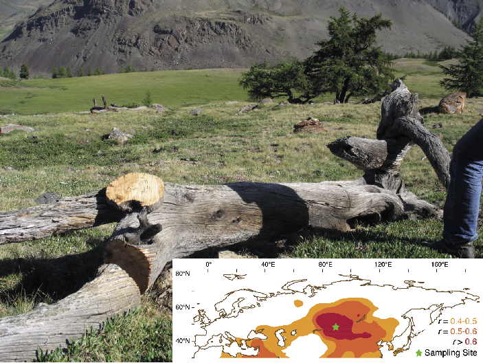
Figure 1: A dry-dead Siberian larch (Larix sibirica Ledeb.) in the Russian Altai Mountains (~88°E, 50°N). The trunk, located well above the current tree line (~2,450m asl), contains several hundred rings and dates back into medieval times (Myglan et al. 2012). Such samples allow to develop an annually resolved and absolutely dated summer temperature reconstruction. The inset shows spatial field correlations of a new Altai tree-ring width record against gridded JJA temperatures from AD 1821-2011. Partners include V.S. Myglan, D.V. Ovtchinnikov and A.V. Kirdyanov (all Krasnoyarsk, Russia). Photo: Myglan VS, Inset: Büngten U unpublished. |
By hosting our workshop, the CESEFOR Foundation (www.cesefor.com) made a considerable contribution to a successful start of Phase 2 of PAGES’ EuroMed2k working group. Soria was selected as location not the least because it is a region on the Iberian Peninsula where a marked drying trend has affected ecosystem functioning and productivity since the 1970s (Büntgen et al. 2012, 2013). As a consequence, some local agriculture foci already shifted from traditional timber harvesting to non-woody forest products, e.g. mushrooms, and irrigation during summer had to be intensified. The underlying processes forcing this climatic trend are, however, not well understood. Gaining further knowledge on such regional climatic patterns is one of the goals of the EuroMed2k working group. Therefore, and considering a broader spatiotemporal perspective, this working group aims at compiling a wide range of proxy data for providing a long-term perspective on the modern climate, performing model-data comparison assessments, and supplementing detection and attribution studies.
A total of 39 scientists from 11 countries with expertise in paleoclimatic data, reconstructions and climate models for the North Atlantic/European/Mediterranean sector and the western part of Russia attended the workshop. In contrast to the first project phase, the interest has changed towards the compilation and evaluation of high- to low-resolution terrestrial and marine proxy archives covering at least some centuries, but ideally several millennia. The workshop participants also acknowledged the value of integrating lower resolution marine records from the Atlantic Ocean and Mediterranean Sea that are longer than 2ka. At the same time, they were aware of the statistical challenges of combining annually resolved and lower resolution timeseries, such as the incorporation of different levels of temporal uncertainty inherent to different proxy archives.
EuroMed2k will extend the initial temperature-oriented proxy compilation towards high-, mid-, and low-resolution terrestrial and marine hydroclimatic archives, and expand the network beyond Eastern Europe including the Caucasus, Polar Ural, and Altai Mountains (Fig. 1). The working group aims to generate a comprehensive paleoclimatic database for the development of at least four independent reconstructions of annual and lower resolution temperature and hydroclimate. Moreover, the most recent generation of Earth System Climate Models, now spanning the last two millennia, incorporate hydrological changes in Europe. Those will allow proxy-model cross-comparison of overlapping periods, in-depth assessments of spectral properties (PAGES 2k Consortium 2014), and testing methods for empirical climate reconstructions in the context of regional-scale pseudo-proxy experiments (Gomez-Navarro et al. in press).
The working group plans to substantially expand the EuroMed2k database: around 70 records will be added, representing different resolutions and covering different age ranges from several centuries to most of the Holocene. The records will cover the area from 25-70°N and 10°W-45°E, with geographical foci on the Iberian Peninsula, Alpine arc, and Fennoscandia. Particular emphasis will be given to so far under-represented marine and terrestrial records of lower resolution to help fill seasonal, temporal, and spatial gaps in the existing network. An extensive compilation of sediment cores from both the North Atlantic and Mediterranean may indeed offer seasonally disjunct information on decadal to multi-millennial time-scales; and speleothems from the Near East (Göktürk et al. 2011) can contain winter signals and cover several millennia.
As a community-driven project, a key success factor of PAGES2k will be its public visibility. We therefore complemented our workshop with a public roundtable at the headquarters of the regional government, where members of the EuroMed2k consortium enthusiastically discussed climate issues with the regional media, representatives of the sylvicultural and agricultural sectors, delegates of the agro-food and myco-touristic industries, and an interested lay audience. PAGES paleoclimatologists were able to place the ongoing Iberian drought in a historical context and compare the regional Spanish conditions with trends in other parts of the world.
affiliations
1WSL, Birmensdorf and OCCR Bern, Switzerland
2Global Change Research Centre, Brno, Czech Republic
3Department of Geography, Justus Liebig University of Giessen, Germany
4Bolin Centre for Climate Research, Stockholm University, Sweden
5Department of Geography, Johannes Gutenberg University, Mainz, Germany
6Department of Archaeology and Centre of Past Climate Change, University of Reading, UK
7Department of Geography, University of Swansea, UK
8Institute of Geoscience, Faculty of Physics, University Complutense Madrid, Spain
9Institute for Coastal Research, Helmholtz Centrum, Geesthacht, Germany
10Department of Earth Science, University of Bergen, Norway
11Research Unit of Forestry Mycology and Trufficulture, Cesefor Foundation, Soria, Spain
contact
Ulf Büntgen: buentgenwsl.ch
references
Büntgen et al. (2012) Nat Clim Change 2: 827-829
Büntgen et al. (2013) Glob Planet Change 107: 177-185
Göktürk et al. (2011) Quat Sci Rev 30: 2433-2445
Gómez-Navarro et al. (in press) Clim Dyn, doi:10.1007/s00382-014-2388-x
Bernd Zolitschka1, P. Francus2,3, A.E.K. Ojala4, A. Schimmelmann5 and C. Telepski6
 |
|
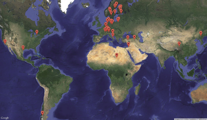
Figure 1: Screenshot from the Varve Image Portal documenting the current global coverage of varve images. |
Annually laminated (i.e. varved) sediment sequences are important natural archives of paleoenvironmental conditions that offer an accurate indication of time span in absolute years, exceptional high (up to seasonal) temporal resolution, and the possibility of calculating sediment flux rates. During the 19th International Sedimentological Congress 2014 in Geneva, Switzerland, a new tool for the dissemination of visualized information from annually laminated sediments – the online Varve Image Portal – was officially launched. This new website displays images of various varve types based on contributions from the scientific community. This online resource is now fully operational and growing and we are asking for input from scientists around the world (Fig. 1). Please contribute your additional varve images from new and published sites together with metadata to Bernd Zolitschka: zoliuni-bremen.de
Improving varve analysis
Although the scientific community has come to appreciate the value provided by both marine and lacustrine annually laminated sediments, there remains a widespread lack of awareness about the need to provide careful evidence that finely laminated sediments are truly varved before exploiting lamina counts for geochronological purposes and environmental interpretations through time.
Such a misconception between varved and finely laminated sediments might partially originate from the history of the expression "varve", a term introduced by the Swedish geologist De Geer during the early 20th century to describe minerogenic proglacial lake sediments of Sweden as annually laminated. Later on, the term varve was extended to other lacustrine as well as marine sediment types with preserved annual successions and seasonal sub-laminae. The large diversity of sediments featuring a varved character sometimes led to the misconception that most, if not all finely laminated sediments must be varved, which clearly is not the case.
The Varve Image Portal aims to provide exemplary visual information regarding the compositional and structural diversity of varved sediments, and to assist, train and guide researchers in the critical judgment of the relative timing of (sub)-laminae and how to constrain their geochronological potential. The Varve Image Portal also intends to disseminate existing image information about varves and to facilitate the efforts of students and young scientists to get acquainted with the challenging topic of finely laminated sedimentary structures. It is accessible via
http://pastglobalchanges.org/science/end-aff/varves-wg/varves-image-library
Using the portal
Each varve image of this online database is accompanied by metadata including information about the study site, satellite and terrestrial images as well as references with DOI links to publications reporting the specific varve record.
The Varve Image Portal has three different search functionalities: (1) A map-based search, (2) a search based on a genetic concept where varves are compositionally categorized as clastic, biogenic, endogenic (incl. evaporitic) and mixed, and (3) an alphabetic search of site names.
This online tool offers exemplary views on many different aspects of varved sediment structures including macroscopic images of gravity and freeze cores. Microscopic images with different magnifications provide examples in normal and polarized light. Scanning electronic microscope images, radiographs and images combined with analytical data or interpretations complete this internet-based resource. Additionally, general information about varves as well as links to varve-related and methodologically relevant websites are provided. Finally, the Varve Image Portal provides easy access to varve reviews, to other iconic publications closely linked to varve studies as well as to publications related to methods and techniques that apply to the investigation of varved sediment records.
affiliations
1Institute of Geography, University of Bremen, Germany
2Institut National de la Recherche Scientifique, Québec, Canada
3GEOTOP-UQAM-McGill, Montréal, Canada
4Geological Survey of Finland, Espoo, Finland
5Department of Geological Sciences, Indiana University, Bloomington, USA
6PAGES International Project Office, Bern, Switzerland
contact
Bernd Zolitschka: zoliuni-bremen.de
Peter Gell1, J. Dearing2, S. Juggins3, M-E Perga4, J. Saros5 and C. Sayer6
Wetlands and water remain a key realm of applied paleoecological research with many proxies reflecting the changing status of the water body as well as reflecting the climatic and human drivers of these changes. This working group will review direct human impact on aquatic ecosystems at times in the past critical to each region and the internal ecological shifts of the wetlands, to explore the responsiveness, resistance, and resilience of aquatic systems worldwide to natural and anthropogenic forces.
Human activities have impacted greatly on global aquatic systems through the release of pollutants and the regulation and abstraction of surface and groundwater. This has, and will continue to impact critically on ecosystem productivity with further consequences for human wellbeing. Simultaneously, aquatic systems have responded to long and shorter-term variations in temperature and effective precipitation.
 |
|
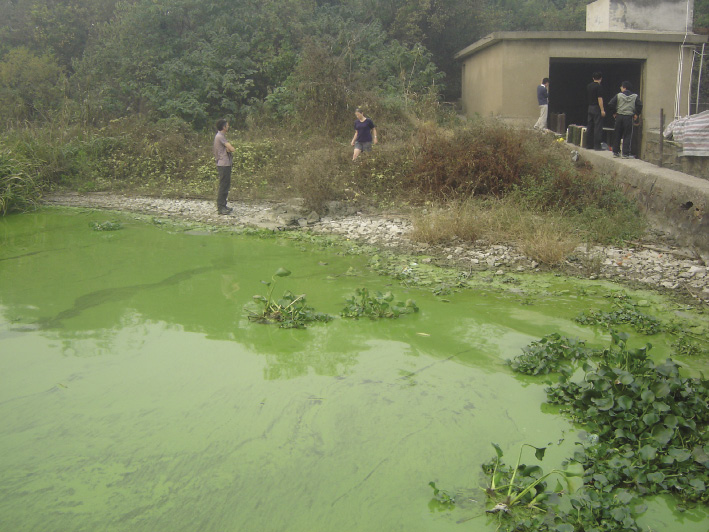
Figure 1: Taihu Lake, on the southern part of the Yangtze River delta, is the third largest freshwater lake in China. Taihu became eutrophic following intensive development from the 1980s and has been covered by an extensive Microcystis bloom since the late 1990s. Understanding the nature of aquatic transitions provides insights for the challenge of wetland restoration. |
Many of these responses have been non-linear, with aquatic ecosystems both responding abruptly, and showing a certain level of resilience to forces until a threshold is breached. Wetlands are a classic ecosystem used to demonstrate alternative stable states whereby feedbacks can act to resist pressures, but also act to entrench the system in a new state once pressures force a regime shift.
Many of the changes witnessed, or modeled, by ecologists have existed in the past. Accordingly, research on major transitions in aquatic systems represents a significant field of enquiry that demands contribution from both contemporary ecology and paleoecology. Further, long term records of change provide evidence of the ecosystem dynamics that may have occurred leading up to a threshold change and, thereby, can reveal early warning signals that may be lessons to prioritise intervention measures for future management.
Scientific goals and activities
The Aquatic Transitions Working Group has two principal charters or projects. The first is to document the global history of the impact of humans on aquatic systems. By identifying the first point of human impact and the inception and peak of the impact of the industrialised phase, Project 1 will reveal the responsiveness of aquatic systems to the presence of humanity, within a framework of climate variability. Project 2 will drill down into the nature of these transitions to examine the ecosystem dynamics that have resisted human pressures, as well as the changes leading up to the point where the system succumbed, and the degree to which new, stabilising forces have entrenched the system in a new regime.
Aquatic Transitions will achieve these goals by collating published global paleohydrological and paleoecological records, sifting through these records and attributing changes in records to critical phases in human settlement and activity. It will select critical points of impact that may be time transgressive. By focussing its research on these points of transition, the working group will apply established ecological reason to attribute the identified changes to press or pulse responses or regime shifts. Thus it will respond directly to several key questions in paleoecology as identified at the PAGES-supported Palaeo50 workshop in 2012 (Seddon et al. 2014).
Aquatic Transitions seeks representation from across the globe and will use meetings to assemble a global database, use change point analysis to identify timing and cause of change, synthesize records at continental and global scales, and write outputs.
Visit the Aquatic Transitions website at: http://pastglobalchanges.org/science/wg/former/aquatic-transitions/intro and sign up to our mailing list to keep up to date with our activities.
Upcoming activities
The first meeting of the Aquatic Transitions Working Group will be in Keyworth, UK, 22-24 April 2015, and there will be a follow up workshop on 3 August 2015 in association with the International Paleolimnology Congress in Lanzhou, China.
affiliations
1Water Research Network, Federation University Australia, Ballarat, Australia
2Geography and Environment, Southampton University, UK
3Geography, Newcastle University, UK
4Institute national de la recherche agronomique, Paris, France
5Climate Change Institute, University of Maine, USA
6Environmental Change Research Centre, University College London, UK
contact
Peter Gell: p.gellfederation.edu.au
reference
News
PAGES 5th OSM and 3rd YSM
Preparations are well underway for PAGES’ flagship event, the Open Science Meeting and associated Young Scientists Meeting, to be held in Zaragoza, Spain, in May 2017.
The YSM runs from 7-9 May and the selection process is competitive. The OSM runs from 9-13 May. Following an open call, 33 sessions have been chosen.
Read more and register: http://pages-osm.org
The social media hashtag for both events will be #PAGES17.
New PAGES domain
Following the end of the International Geosphere-Biosphere Programme (IGBP) in December 2015, PAGES’ new domain name is www.pastglobalchanges.org. We encourage everyone to resave old bookmarks.
New PAGES' working groups
Five new working groups have recently been launched:
- • Forest Dynamics http://pastglobalchanges.org/ini/wg/forest-dynamics/intro
- • Climate Variability Across Scales (CVAS) http://pastglobalchanges.org/ini/wg/cvas/intro
- • Global Paleofire 2 (GPWG2) http://pastglobalchanges.org/ini/wg/gpwg2/intro
- • Paleoclimate Reanalyses, Data Assimilation and Proxy System modeling (DAPS) http://pastglobalchanges.org/ini/wg/daps/intro
- • Resistance, Recovery and Resilience in Long-term Ecological Systems (EcoRe3) http://pastglobalchanges.org/ini/wg/ecore3/intro
Read more about Forest Dynamics, CVAS and Global Paleofire 2 in their Program News articles in this issue, and read about all groups on our website. All PAGES' working groups are open for participation to interested scientists.
PAGES' SSC meeting 2016 and new SSC members
PAGES’ Scientific Steering Committee (SSC) met in Cluj-Napoca, Romania, in May 2016. PAGES’ two-day Central and Eastern Europe Paleoscience Symposium followed the SSC meeting.
At the end of 2016, co-chair Hubertus Fischer and Claudio Latorre finish their tenures, and we take this opportunity to thank them for their commitment throughout their two terms.
We welcome the two new incoming members starting January 2017:
- • Willy Tinner - head of paleoecology at the University of Bern’s Institute of Plant Sciences, Switzerland. His department addresses ecological and climatic questions on annual to millennial time scales and uses quaternary sedimentary sequences (e.g. pollen, macrofossils, charcoal, diatoms, chironomids) and modeling approaches to study the long-term interactions among climate, the biosphere and society. Tinner will also be PAGES' co-chair.
- • Ed Brook - geology program director at the College of Earth, Ocean, and Atmospheric Sciences at Oregon State University, USA. He specializes in paleoclimatology and geochemistry plus ice-core trace gas records, cosmogenic isotopes and extraterrestrial dust.
PAGES at AGU 2016
PAGES' working groups have organized sessions at the AGU Fall meeting in San Francisco this December. For a full list, go to the calendar entry: http://pastglobalchanges.org/calendar/upcoming/127-pages/1458-agu-fall-meeting-2016
Apply for meeting support or suggest a new working group
Each year, PAGES supports many workshops around the world. We also have an open call for new working groups. The next deadline is 10 October 2016. Read more about workshop support and working group proposals here: www.pastglobalchanges.org/my-pages/introduction
Help us keep PAGES' People Database up to date
Have you changed institutions or are you about to move? Please check if your details are current. http://pastglobalchanges.org/people/people-database/edit-your-profile
Upcoming issues of PAGES Magazine
The next issue of PAGES Magazine will be on climate change and cultural evolution. Contact Claudio Latorre (clatorrbio.puc.cl) now if you wish to contribute to this issue.
The following issue will be on biodiversity and guest edited by our SSC members Lindsey Gillson (lindsey.gillsonuct.ac.za) and Peter Gell (p.gellfederation.edu.au). Contact them or the PAGES office if you are interested in contributing.
In general, if you wish to lead a special section of the magazine on a particular topic, contact the PAGES office or speak with one of our SSC members. http://pastglobalchanges.org/about/structure/scientific-steering-committee
Calendar
2nd QUIGS workshop
18-20 October 2016 - Montreal, Canada
Past land-cover change in Latin America
29-30 October 2016 - Salvador de Bahia, Brazil
1st CVAS workshop
28-20 November 2016 - Hamburg, Germany
Fire and land-cover changes in Europe
5-8 December 2016 - Frankfurt, Germany
PAGES 5th OSM and 3rd YSM
7-13 May 2017 - Zaragoza, Spain
2nd VICS workshop
8 May 2017 - Zaragoza, Spain
www.pastglobalchanges.org/calendar
Featured products
PIGS
The final product from the former working group PIGS (now morphed into QUIGS), “Interglacials of the last 800,000 years” is a mammoth undertaking (2016, Rev Geophys 54).
2k Network
• Charpentier Ljungqvist et al. discuss how rainfall patterns have changed during the 20th century compared with the last twelve centuries (2016, Nature 532).
• McKay and Emile-Geay set out their plans for a Linked Paleo Data (LiPD) framework (2016, Clim Past 12).
• Huge media interest surrounded the Euro-Med2k consortium paper on European summer temperatures (2016, Env Res Lett 11).
• Recent temperatures experienced in Australia and New Zealand are warmer than any other 30-year period over the past 1,000 years (Gergis et al. 2016, J Climate 29).
PALSEA2
• Editorial by Stockholm Resilience Centre Director Johan Rockström highlights the quality of work done by the PALSEA working group, and PAGES in general. He also discusses the importance of our parent organization Future Earth and summarizes the legacy of the IGBP (2016, Science 351).
• Assessing the impact of fossil corals on studying past sea-level change (Hibbert et al. 2016, Quat Sci Rev 145).
Special Issues from PAGES-supported meetings
• "Mediterranean Holocene Climate, Environment and Human Societies" from a meeting in Greece in 2014 (2016, Quat Sci Rev 136).
• “Understanding Change in the Ecological Character of Internationally Important Wetlands” is the outcome of a 2013 meeting in Australia (2016, Mar Freshwater Res 67).
Cover
Where the Greenland Ice Sheet meets the North Atlantic
Icebergs in high summer in Sermilik Fjord, one of the largest fjords in southeast Greenland. Helheim Glacier, which drains into the fjord, has seen some of the highest acceleration of ice velocity recorded across the Greenland Ice Sheet over the past decade (credit C.J. Fogwill).
Chris S.M. Turney1, C.J. Fogwill1, T.M. Lenton2 and R.T. Jones2
Many natural and human systems are vulnerable to long-term forcing that can push them into a different mode of operation. The “tipping points” where such abrupt changes occur are notoriously hard to predict. Looking ahead, a key problem for reducing the uncertainty in future projections is that historical records of change are too short to test the skill of the current generation of climate and environmental models, raising concerns over our ability to successfully predict abrupt change and plan for it. Published records only allow a robust reconstruction of global temperature back to 1880 and show a long-term increase of 0.85˚C. At regional scales, there have been some abrupt changes within the instrumental record. Looking further back in time, a wealth of geological, chemical and biological records capture large-scale, abrupt and often irreversible (centennial to millennial in duration) shifts in environmental and climate systems, providing an opportunity to better understand and therefore predict potential future changes.
 |
|
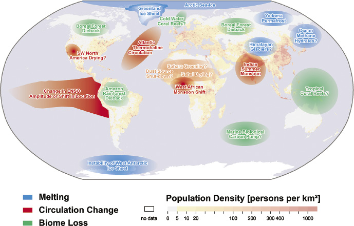
Figure 1: Map of potential policy-relevant tipping elements in the climate system overlain on global population density. Question marks indicate systems whose status as policy-relevant tipping elements is particularly uncertain. Figure by Veronika Huber, Martin Wodinski, Timothy M. Lenton and Hans Joachim Schellnhuber. |
The forcing associated with these changes in the past appears to have been relatively small, implying the existence of underlying tipping points where self-propelling change – i.e. strong, positive feedback – is triggered within the systems in question. Many regions of the world are now recognized as potentially highly-sensitive to abrupt changes caused by the passing of tipping points within different components of the climate system (Fig. 1). Some are of global significance, such as the collapse of the West Antarctic and Greenland ice sheets (leading to a sea level rise of several meters) or reorganization of the Atlantic Meridional Overturning Circulation (AMOC), and corresponding southward shift in the inter-tropical convergence zone of rainfall. Others are of more regional importance, such as the greening of the Sahara.
Innovative analyses of high-resolution records of past change suggest the climate system characteristically slowed down when a tipping point was approached. This raises the prospect that science may be able to provide society with early warning of future approaching tipping points. However, to do this successfully for inherently “slow” components of the Earth system, such as the AMOC and ice sheets, will require high-resolution paleo reconstructions of the variability of these systems in the run-up to the industrial era – providing a new motivation for PAGES' research. In addition, accurate reconstructions of the past behavior of climatic, environmental and archeological systems on quantified, absolute-dated and robust timescales provide the opportunity to better understand the underlying mechanisms and test models of future change.
This Past Global Changes Magazine describes developments in modeling past tipping points and human systems to better understand future change. Reflecting the nature of tipping points within the Earth system, the articles presented reflect a range of truly multidisciplinary research, which crosses traditional time periods or horizons. We hope the selected articles provide valuable insights into the role that tipping points play in understanding past change, and, importantly, highlight the potential of tipping points to provide lessons from the past that will help define the future.
affiliations
1Climate Change Research Centre, University of New South Wales, Australia
2Department of Geography, University of Exeter, UK
contact
Chris Turney: c.turneyunsw.edu.au
Zoë A. Thomas1 and Richard T. Jones2
The analysis of paleo-environmental archives provides a mechanism for identifying systems vulnerable to abrupt change or “tipping points”. Perturbations to natural systems, so-called “stochastic noise”, can play a significant role in understanding past and future variability.
Abrupt changes or “tipping points” in environmental systems are often characterized by a nonlinear response to gradual forcing, and may have severe and wide-ranging impacts, including an irreversible shift to a new state (on human timescales). Arguably one of the best ways to identify and potentially predict threshold behavior in environmental systems is through the analysis of natural archives (paleo records). Generic rules can be used to identify early warning signals that may be identified on the approach to a tipping point, generated from characteristic fluctuations in a time series as a system loses stability.
Recently developed methods to detect these early warning signals exploit a phenomenon called “critical slowing down”. This phenomenon predicts that as a system nears a tipping point, the recovery time to its initial equilibrium after a perturbation should increase. This increase in recovery time can be measured as increasing autocorrelation and variance over a sliding window (Kleinen et al. 2003; Lenton et al. 2012). With the popularity of the free statistical software “R”, this analysis is becoming increasingly applied by the paleo community to understand mechanisms of change (for instance, Early-Warning-Signals Toolbox at http://cran.r-project.org/web/packages/earlywarnings/earlywarnings.pdf). Time-series precursors from natural archives thus have a great potential to enhance our understanding of past abrupt change and provide a means of forewarning potential tipping points. Critical in this regard is recognizing that different rates of forcing significantly influence the temporal resolution required to identify such forewarnings in paleo-environmental time series.
Linking theory to the past
While previous studies have demonstrated the value of natural archives for identifying tipping points (e.g. Dakos et al. 2008), considerable scope exists to expand this work. A major challenge is that paleoenvironmental data typically have high noise levels and a low sampling resolution, whereas theoretical early warning indicators assume only weak stochastic disturbances. When systems are characterized by high levels of stochastic noise, early warning signals may not always detect the approach of a bifurcation (defined as the point at which a system exits its stable equilibrium), since high levels of noise can mask the signal of critical slowing down.
Although the efficacy of the leading indicators (autocorrelation and variance) has been interrogated using a long time series with low noise levels (Dakos et al. 2012), the predictive ability of these indicators with strong noise and a low sampling resolution has been less well studied. Ecological literature, however, has led the way in this regard. The importance of environmental variability in the modeling of ecological systems was first emphasized by Holling (1973), who noted that stochastic noise reduced the resilience of a system. Similarly, analysis of the leading early warning indicators using a multi-species model (Carpenter and Brock 2004) found that both increased noise intensity and decreased sampling rate were found to have a strong negative effect on the ability to detect early warning signals of an impending shift (Perretti and Munch 2012).
 |
|
Figure 1: Typical behavior of systems with (A) low and (B) high noise levels, and (C) an example of flickering. |
Simple bifurcation models can be used to illustrate the role of stochastic noise. It is important to note that the bifurcation point (where intrinsic stability properties of a system changes) and the point at which the system actually tips are not always the same; high noise levels often tip the system before the bifurcation point is reached (Kleinen et al. 2003). Figure 1 depicts the effect of noise on the timing of the abrupt change, showing that (1) the point of tipping varies much more with a higher noise level, and (2) the point of tipping generally occurs much earlier. Early warning signals tend to be much stronger with reduced noise intensity, when the system tends to tip closer to the bifurcation point. When the noise level is too high, the system may not have time to recover from the perturbations and thus the signals of critical slowing down may not be detected.
Critical slowing down or flickering?
When multiple stable states exist and if stochastic forcing is strong enough, the system can “flicker” back and forth between two basins of attraction as the system reaches this bistable region before the bifurcation (Scheffer et al. 2009; e.g. Fig. 1c). This can be seen in the behavior of lakes prior to a switch from oligotrophic to eutrophic conditions, observed as short-term eutrophication events and algal blooms before a more long-term switch (e.g. Wang et al. 2012). Importantly, many studies which give empirical evidence of critical slowing down do so under a small amplitude of noise, which allows the system to display critical slowing down rather than flickering (Dakos et al. 2013), but is generally unrealistic in paleoenvironmental systems. Since “flickering” seems to occur when there is a high noise level, this behavior is probably more prevalent in climate systems than first thought.
An appreciation of the number of states within the system can be beneficial to understand the underlying dynamics of a system. For some time series, this can be visually obvious or is pre-determined by a theoretical model, such as Stommel’s two box model of the thermohaline circulation (Stommel 1961). The exact number of states in a system is sometimes difficult to determine by eye, however, particularly when there are more than two states present. Potential analysis is a technique that can be used to determine the number of states in a system over time, by reconstructing the changing state-space of a system through the modality of the data distribution (Livina et al. 2010). In systems with a relatively high level of noise, if there are multiple stable states present, the system is likely to sample these states over time and this represents a kind of flickering in the system (Dakos et al. 2012).
Multiple stable states: A case study
 |
|
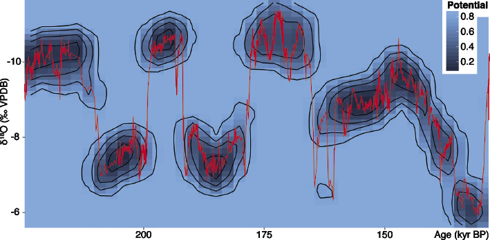
Figure 2: Visualization of the potential function derived from the speleothem δ18O data (overplotted in red; x-axis inverted), showing the presence of multiple stable states (Wang et al. 2008; Thomas et al. 2015). The potential function gives an intuitive picture of the stability of the system, where darker blue indicates a deeper, more stable potential, and the lighter blue areas an unstable region of the potential basin. |
The techniques described above have been used in the analysis of speleothem sequences from China to gain an understanding of the mechanisms of abrupt changes in the Asian monsoon system (Thomas et al. 2015). Figure 2 shows the δ18O values from a speleothem from Sanbao Cave in China (Wang et al. 2008), spanning the penultimate glacial cycle. More negative δ18O values indicate higher rainfall amount (strong monsoon), while less negative δ18O values indicate lower rainfall amount (weak monsoon), over millennial timescales. Potential analysis undertaken on this data shows that the system jumps between different stable states (indicated by the darker blue areas in Fig. 2), from a strong monsoon state to a weak monsoon state and vice versa. This is particularly prominent during the older half of the record.
Conclusion
The recognition of multiple stable states in natural archives provides a powerful means of understanding Earth system dynamics. The ability to identify periods in the past where thresholds have been crossed is critical if we are to predict and avoid dangerous abrupt climate change in the future.
Acknowledgements
This work is supported by the Australian Research Council Laureate Fellowship (FL100100195). Thanks to Chris Turney and Tim Lenton for help editing this paper.
affiliations
1Climate Change Research Centre, University of New South Wales, Sydney, Australia
2Department of Geography, University of Exeter, UK
contact
Name: z.thomasunsw.edu.au
references
Carpenter SR, Brock WA (2004) Ecol Soc 9: 8-38
Dakos V et al. (2008) PNAS 105: 14308-14312
Dakos V et al. (2012) PLoS One 7, doi:10.1371/journal.pone.0041010
Dakos V et al. (2013) Theor Ecol 6: 309-317
Holling CS (1973) Annu Rev Ecol Syst 4: 1-23
Kleinen T et al. (2003) Ocean Dyn 53: 53-63
Lenton TM et al. (2012) Phil Trans Roy Soc Math Phys Eng Sci 370: 1185-1204
Livina VN et al. (2010) Clim Past 6: 77-82
Perretti CT, Munch SB (2012) Ecol Appl 22: 1772-1779
Scheffer M et al. (2009) Nature 461: 53-59
Stommel H (1961) Tellus 13: 224-230
Thomas ZA et al. (2015) Clim Past 11: 1621-1633
Michel Crucifix
Simple models formulated in the 1960s started a research tradition focused on stability and transitions in the climate system. Later, climate scientists realized the importance of stochasticity. What do these concepts imply for ice ages today?
In 1969, M.I. Budyko in Russia and W.D. Sellers in the US published two very similar studies. From reasoning about the energy balance of the Earth's system, they found that comparatively small variations of atmosphere transparency (Budyko) or in solar constant (Sellers) would be enough to drive the Earth into an ice age. Their key discovery was that Earth's climate could exhibit two steady states. Earlier that decade, Stommel (1961) deduced the existence of irreversible transitions between two thermohaline circulation structures in a simple model of abyssal water flow. Now we also think that vegetation-atmosphere coupling can lead to multiple states (Brovkin 1998).
The existence of multiple steady states leads naturally to the concept of “tipping”. Within a state, a system is largely self-stabilizing, but too large a perturbation may shift it into another self-stabilizing state, with little probability of escaping back to the original state. The ideas behind the models of Budyko, Sellers and Stommel provided a basis to interpret a range of paleoclimate events, including glacial inception, Heinrich events, and the end of African Humid Period.
What about the deglaciation? In a quite mathematical but pioneering article, Saltzman and Verbitzky (1993) pointed out that two possible destabilization mechanisms could be at play: the mechanical collapse of Northern Hemisphere ice sheets and the abrupt release of CO2 accumulated in the deep ocean to the atmosphere. These two processes are still considered relevant today (Abe-Ouchi et al. 2013; Paillard and Parrenin 2004)
Tipping to ping pong
Is the deglaciation, however, really the consequence of passing a “tipping point”? Or, to paraphrase Crowley (2002), are we looking obsessively for "tipping, tipping everywhere"?
 |
|
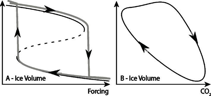
Figure 1: Two examples of conceptual models for paleoclimate dynamics. (A) The Budyko-Sellers model envisions two stable states for a range of forcing. Large forcing deviations from the resting state may precipitate a transition; (B) In a limit cycle, glacial interglacial stages succeed each other as a result of internal dynamics, without the need for forcing. In this case, insolation forcing is but a pacemaker that controls the timing of transitions. |
Models such as Stommel’s feature a specific mathematical property, known in the specialized literature as a "fold bifurcation". It is a common feature of non-linear systems that fits well with the idea that a slow change in environmental conditions can induce a rapid and irreversible transition towards a new state once a "threshold" is crossed (Fig. 1A). However, this is only one of a very rich set of possibilities. For example, in the Paillard-Parrenin model (2004), a glacial maximum is inherently unstable, and CO2 outgassing ejects the system toward an interglacial. A background glaciation process then brings the system back to a glacial state, from where it is ejected again. In this model, the glacial-interglacial process no longer requires an externally forced tipping: it is the manifestation of a self-sustained oscillation, also known as a limit cycle. Instead of tipping, this (Fig. 1B) is ping pong!
Accounting for Randomness
Fold bifurcations and limit cycles are examples of concepts defined by a branch of mathematics called "dynamical systems theory". Since the 1960s, this discipline has provided climate scientists with an inexhaustible framework for depicting, characterizing and hypothesizing about possible system transitions and cycles. Ghil (1976) wrote one of the pioneering papers on the subject. More recently, Crucifix (2013), and Aswhin and Ditlevsen (2015) have analyzed models akin to those shown in Figure 1 in the context of ice ages.
 |
|
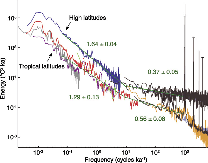
Figure 2: Estimate of the energy spectrum from annual to astronomical scales, adapted from (Huybers and Curry 2006). Numbers in green are spectral slopes on the logarithmic plot. All time scales may potentially interact: there is no gap between astronomical and centennial time scales. |
Such models represent a very small class of possibilities. In particular, they are "deterministic": the trajectory is entirely determined by original conditions and forcing. Since the seventies, however, climate scientists have realized that this framework needs to be extended. The problem is that spectral analysis shows that the climate system varies on all timescales (Fig. 2), yet deterministic models always neglect a part of this spectrum. So we need, somehow, to account for the unresolved fluctuations to realistically represent dynamical effects.
This is where stochastic theory can help. A stochastic quantity is a mathematical concept used to represent a variable which is not known precisely, but which can be described in terms of probability distributions. The idea is to account for atmospheric variability with a stochastic process taking different random values with time (Hasselman 1976; Saltzman 1981).
This leads to an interesting mathematical problem: what happens to tipping points when stochastic terms are included? With small amounts of stochasticity, the system may exhibit "early warning signals" before a transition: a valuable property, indeed, if we want to predict the occurrence of a large transition. In some cases, however, the presence of stochastic components modifies the structure of the deterministic model so drastically that the tipping point completely vanishes. In this case, systems like the one depicted in Figure 1 lose their relevance. We do not know whether this scenario applies to ice ages, but in some models even small amounts of stochasticity can substantially modify the timing of ice ages (Ditlevsen 2009; Crucifix 2012).
Some will say that Nature isn't "chaotic", "deterministic", or "stochastic". These properties only apply to models. What mathematics has to offer us is the ability to characterize the model which, among alternatives, best explains the data at hand about the real world. If this best model presents tipping points, then we can take decisions accordingly.
Identifying a “best” model among alternatives is a problem that can be framed statistically. In general, statistics work best with models that do not include too many parameters. A simple model is also easier to analyze and characterize. This is why there is still a research tradition focused on conceptual models similar to those of Figure 1.
However, our knowledge of environmental systems relies also on complex numerical models, which allow us to infer emergent constraints on the basis of physical laws of ice, atmospheric and oceanic motion, and such models tend to include hundreds of parameters. A key challenge for climate scientists is thus to articulate models of different levels of complexity within a consistent framework, from the conceptual models to the complex numerical codes.
A challenge for the decade
Stochastic theory may again provide a way forward. Stochastic parameterizations of interannual and interdecadal variability could be developed on the basis of experiments with general circulation models. Such parameterizations could then be included in models of intermediate complexity (EMICs) to estimate the effects of interdecadal variability on the slower modes of motion. This would provide a means to model the cascade of variability effects, from interannual to ice-age time scales: a revolution with respect to modern practices. Whether such stochastic EMICs will still present tipping points similar to those depicted on Figure 1 is an important question waiting to be answered.
affiliation
Earth and Life Institute, Université catholique de Louvain, Louvain-la-Neuve, Belgium
contact
Michel Crucifix: michel.crucifixuclouvain.be
references
Abe-Ouchi A et al. (2013) Nature 500: 190-193
Ashwin P, Ditlevsen P (2015) Clim Dyn 45: 2683-2695
Budyko MI (1969) Tellus 21: 611-619
Brovkin V et al. (1998) J Geophys Res 103: 31613-31624
Crowley TJ (2002) Science 295: 1473-1474
Crucifix M (2012) Phil Trans R Soc A 370: 1140-1165
Crucifix M (2013) Clim Past 9: 2253-2267
Ditlevsen PD (2009) Paleoceanography 24, doi:10.1029/2008PA001673
Ghil M (1976) J Atmos Sci 33: 3-20
Hasselmann K (1976) Tellus 28: 473-485
Huybers P, Curry W (2006) Nature 441: 329-332
Paillard D, Parrenin F (2004) Earth Planet Sci Lett 227: 263-271
Saltzman B et al. (1981) J Atmos Sci 38: 494-503
Sellers WD (1969) J Appl Meteo 8: 392-400
Saltzman B, Verbitsky MY (1993) Clim Dyn 9: 1-15
Christopher J. Fogwill1, N.R. Golledge2,3, H. Millman1 and C.S.M. Turney1
Sea-level reconstructions suggest significant contributions from the East Antarctic Ice Sheet may be required to reconcile high interglacial sea levels. Understanding the mechanism(s) that drove this loss is critical to projecting our future commitment to sea-level rise.
The stability of the Antarctic ice sheets and their potential contribution to sea level under projected future warming remain highly uncertain. In part, this uncertainty arises from comparison with past interglacial periods when, despite only small apparent increases in mean atmospheric and ocean temperatures, eustatic sea levels are interpreted to have been 5-20 meters higher than present (e.g. Dutton et al. 2015). To achieve these highstands, undefined mechanisms or feedbacks that substantially increased the net contribution of the Earth’s ice sheets to global sea level must have been at work. Understanding the feedbacks and tipping points that drove sea-level rise during past interglacial periods are therefore not only key to improving sea-level projections over the next century, but critically, given that ice-sheet response times are far longer than those of the atmosphere or ocean, they are important for quantifying our commitment to ice loss and sea-level rise over millennia.
Last Interglacial sea levels
The Last Interglacial (LIG; 135,000-116,000 years ago) is a key period in this regard; described as a “super-interglacial”, empirical evidence suggests that the LIG was only around 2°C warmer than pre-industrial times, whilst sea levels were far higher (Turney and Jones 2010). Critically, the LIG was associated with an early rate of global sea-level rise that exceeded 5.6 meters per kyr, culminating in global sea levels 6.6-9.4 meters above present (Kopp et al. 2009). At present, the LIG eustatic sea-level-rise budget remains unresolved. Recent reassessments of potential contributions, including ocean thermal expansion (McKay et al. 2011) and wasting of the Greenland and West Antarctic ice sheets, leaves some 0.8 to 3.5 meters of global mean sea level (GMSL) unaccounted for during the LIG. To date, research and media attention has largely focused on the West Antarctic Ice Sheet (WAIS), however the question over the possible contribution made by the far larger East Antarctic Ice Sheet (EAIS) has been raised by both recent contemporary observations (e.g. Greenbaum et al. 2015) and ice-sheet model simulations (e.g. Golledge et al. 2015; Deconto and Pollard. 2016). This raises an important question: might hitherto unidentified mechanisms or feedbacks have induced accelerated mass loss from marine-based sectors of the EAIS?
Ice-sheet model simulations
Global and regional model-based ocean-atmosphere simulations for both future and paleoclimate scenarios are the most powerful tools currently available for establishing both the spatial pattern and variability of environmental perturbations through time, as well as the likely magnitudes of change. This is especially true when such models are empirically constrained, for example, by the verification of model outputs against geological proxy data.
However, to establish likely sea-level changes that may take place under warmer-than-present conditions (either during past interglacials or in the future), it is necessary to employ numerical models capable of accurately simulating the major ice sheets. Together, the Greenland and Antarctic ice sheets act as reservoirs, whose combined freshwater storage capacity must account for the majority of interglacial sea-level variability. The two main ice sheets of Antarctica, the West and the East Antarctic ice sheets contain ~3.9 and ~51.6 m sea-level-equivalent ice volume respectively, thus even relatively small changes in their extents and thicknesses may lead to global sea-level changes of several meters. In Antarctic terms, changes in ice-sheet extent over paleoclimate timescales are primarily controlled by oceanic conditions (Joughin et al. 2012), but in both paleo and future ice-sheet model simulations, inter-model discrepancies may arise because of the manner in which key processes are implemented and parameterized, or the spatial resolution at which experiments are run (Favier et al. 2014).
New directions
Uncertainties over the sources of sea-level rise during the LIG have driven an increased interest in paleo-ice-sheet model simulations, because empirical data exist with which the models can be “ground-truthed”, in contrast to forward projections that are unconstrained. Recent studies have highlighted that the Antarctic ice sheets may be highly sensitive to circulation changes in the Southern Ocean triggered by changes in circulation patterns driven by anthropogenic warming over the next century (Hellmer et al. 2012). To explore the effect that atmospheric circulation changes may have on marine-based sectors of the Antarctic ice sheets during the LIG, Fogwill et al. (2014) examined the role that physical changes in the location of the Southern Hemisphere westerly winds could play in driving WAIS and EAIS change through changing Southern Ocean circulation using Earth System Climate Models (ESCMs). Simulations demonstrated that sectors of the EAIS found to be most sensitive include the Eastern Weddell Sea, the Amery/Lambert region and the western Ross Sea, which when combined could add 3-5 m to GMSL (Fig. 1). Whilst ESCMs provide useful insights into broad scale ocean changes, Regional Ocean Models (ROMs) may prove critical to connect the ice sheet to broad scale ocean circulation changes (e.g. Hellmer et al. 2012).
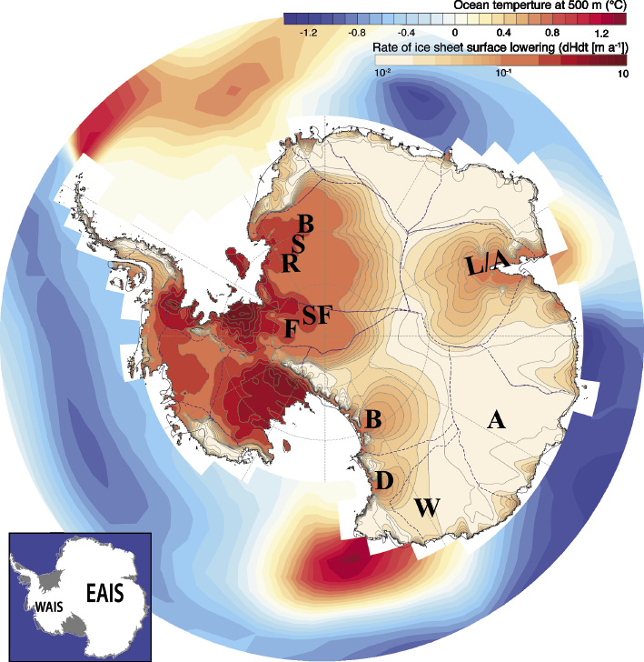
Figure 1: Southern Ocean temperature anomalies at 500 m depth under 135 ka BP boundary conditions with the Southern Hemisphere Westerlies shifted south (for a Southwards shift Southern Hemisphere westerly winds minus control simulation), together with the pattern of ice-sheet thinning from an independent glacial-interglacial ocean-forcing model experiment using the Parallel Ice Sheet Model (PISM) at 5 km resolution. The major EAIS drainage basins are marked F: the Foundation, SF: Support Force, R: Recovery, S: Slessor, B: Bailey basins, L/A: the Ambert/Amery basin, B: the Byrd, D: David, W: Wilkes, and A: Aurora. Inset Map of the Antarctic Continent showing WAIS and EAIS. Adapted from Fogwill et al. (2014).
Paleo-ice-sheet experiments have also been used to explore the possible drivers and mechanisms of EAIS change during past interglacials to provide insights into the future. In one such study, Mengel and Levemann (2014) demonstrated that it is possible to drive self-sustained discharge of the entire Wilkes Basin simply by removing a specific coastal ice volume (termed an ice plug). The GMSL equivalence of such a collapse is on the order of 3-4 m, but the question of how this ice plug could be removed remains unresolved.
One potential scenario involves catastrophic glaciological changes such as ice-shelf hydrofracture and ice-cliff failure. Pollard et al (2015) implemented these two mechanisms on a whole-Antarctic ice-sheet scale for climatic conditions representative of the warm Pliocene. The results of these simulations are dramatic, driving rapid ice-sheet collapse across huge areas of the WAIS and EAIS on centennial timeframes, and producing GMSL equivalence in excess of ~17 m within millennia (Fig. 2). Whilst the mechanisms are highly parameterized, together ice-shelf hydrofracture and ice-cliff failure provide potential “missing links” in the current generation of ice-sheet models (DeConto and Pollard 2016). They are therefore important candidates for future process studies, given that when combined, their effect is far greater than the sum of their individual effects – it is such strong nonlinearities that are the hallmark of a tipping element. Similarly, there is a need to include more accurate simulation of basal hydrological processes at the ice-sheet scale (Bueler and van Pelt 2015), or the ability for changes in basal friction to effect changes in ice-sheet behavior (Golledge et al 2015).
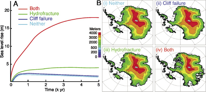
Figure 2: (A) Global mean equivalent sea-level rise in Pliocene warm-climate simulations. Time series of global mean sea-level rise above modern are shown, implied by reduced Antarctic ice volumes. The calculation takes into account the lesser effect of melting ice that is originally grounded below sea level. Cyan: with neither cliff failure nor melt-driven hydrofracturing active. Blue: with cliff failure active. Green: with melt-driven hydrofracturing active. Red: with both these mechanisms active. (B) Ice distribution across the Antarctic continent with (a) neither cliff-failure or melt-driven hydrofraturing, (b) cliff failure active, (c) Melt-driven hydrofrature, and (d) both cliff failure and hydrofracturing incorporated to model simulations equilibrated after 5,000 years of warm-climate forcing. Demonstrating the marked loss of EAIS outlets under scenario d incorporating both cliff failure and hydrofracture. Adapted from Pollard et al. (2015), reprinted with permission of Elsevier.
Conclusions
To understand and quantify the potential of the EAIS as a major tipping element in the Earth's climate system, future developments are needed so that ice-sheet models incorporate the complex interactions between ice sheets and their beds, their connection to ice shelves, and also the continental- and local-scale atmospheric and oceanic forcings that the ice sheets are exposed to (e.g. Bracegirdle et al. 2015). Simulating more realistic ice-flow behavior to external drivers is key if we are to robustly model the response of the Antarctic ice sheets to future changes both at the periphery and the bed. With emerging evidence that the EAIS may be highly susceptible to ocean forcing (Greenbaum et al. 2015), and the concept of marine-ice-sheet instability becoming increasingly accepted and well understood, parameterizing the non-linear mechanisms occurring at the ice-ocean interface is essential if we are to reduce uncertainty in future sea-level rise projections.
affiliations
1Climate Change Research Centre, University of New South Wales, Sydney, Australia
2Antarctic Research Centre, Victoria University of Wellington, New Zealand
3GNS Science, Lower Hutt, New Zealand
contact
Christopher J. Fogwill: c.fogwillunsw.edu.au
references
Bracegirdle TJ et al. (2015) BAMS 97: ES23-ES26
Bueler E, van Pelt W (2015) Geosci Model Dev 8: 1613-1635
Dutton A et al. (2015) Science 349, doi: 10.1126/science.aaa4019
DeConto RM, Pollard D (2016) Nature 531: 591-597
Favier L et al. (2014) Nature Clim Change 4: 117-121
Fogwill CJ et al. (2014) J Quat Sci 29: 91-98
Golledge NR et al. (2015) Nature 526: 421-425
Greenbaum JS et al. (2015) Nature Geosci 8: 294-298
Hellmer HH et al. (2012) Nature 485: 225-228
Joughin I et al. (2012) Science 338: 1172-1176
Kopp RE et al. (2009) Nature 462: 863-867
McKay NP et al. (2011) Geo Res Lett 38, doi:10.1029/2011GL048280
Mengel M, Leverman A (2014) Nature Clim Change 4: 451-455
Pollard D et al. (2015) Earth Plan Sci Lett 412: 112-121
Turney CSM, Jones RT (2010) J Quat Sci 25: 839-843
Summer K. Praetorius1 and Alan C. Mix2
Rapid Northern Hemisphere warming during the last deglaciation involved synchronization of the North Pacific and North Atlantic. Threshold-like transitions to hypoxia occurred in conjunction with abrupt ocean warming, implying synergistic ocean heat transport triggered both physical and ecological tipping points.
The rapid warming transitions into the Bølling-Allerød interstadial and Holocene interglacial are striking examples of nonlinearities in the climate system. A leading hypothesis for the trigger of these events has been changes in the strength of the Atlantic Meridional Overturning Circulation (AMOC) (McManus et al. 2004). However, records from the North Pacific and other distant locations document equally abrupt climate changes as those observed in the North Atlantic (Hendy and Kennett 1999; Wang et al. 2001; Praetorius and Mix 2014). This calls into question whether these are teleconnected responses to changes in the AMOC, or whether they involve orchestration of northern hemisphere climate dynamics and reflect critical transitions in the climate system, possibly involving multiple “tipping elements” (Lenton et al. 2008).
Proposed early warning signals (EWS) of tipping points include enhanced spatial correlation, increased autocorrelation, and high variance (Dakos et al. 2010; Scheffer et al. 2012). Evidence for enhanced variance and autocorrelation prior to the Bølling-Allerød and Holocene transitions is mixed, leading to debate as to whether these abrupt climate shifts are stochastic perturbations or climate bifurcations (Lenton et al. 2012). High spatial correlation may be a more reliable EWS (Dakos et al. 2010), but so far has not been widely applied to paleoclimate data. Detection of EWS in paleoclimate data remains challenging due to requirements for records with high signal-to-noise ratios and precise chronologies.
North Pacific – North Atlantic climate flip-flop?
We recently developed a decadal-resolution planktonic oxygen isotope record from the Gulf of Alaska with a centennial-scale radiocarbon chronology (Praetorius and Mix 2014) and compared changes to the Greenland NGRIP oxygen isotope record (Rasmussen et al. 2006). The two regions appear to flip-flop between correlation and anticorrelation (Fig. 1). A few hundred years prior to the abrupt warming transition into the Bølling-Allerød warm period at 14.7 ka, these records became synchronized, and maintained high correlation throughout the remainder of the deglaciation, encompassing abrupt climate fluctuations such as the Younger Dryas cooling episode and the rapid warming into the Holocene. Coupling of North Pacific and North Atlantic heat transport could act as an amplifying mechanism in abrupt northern hemisphere climate change, whereas opposing oceanic regimes could act to balance northern hemisphere heat transport, and thus promote climate stability.
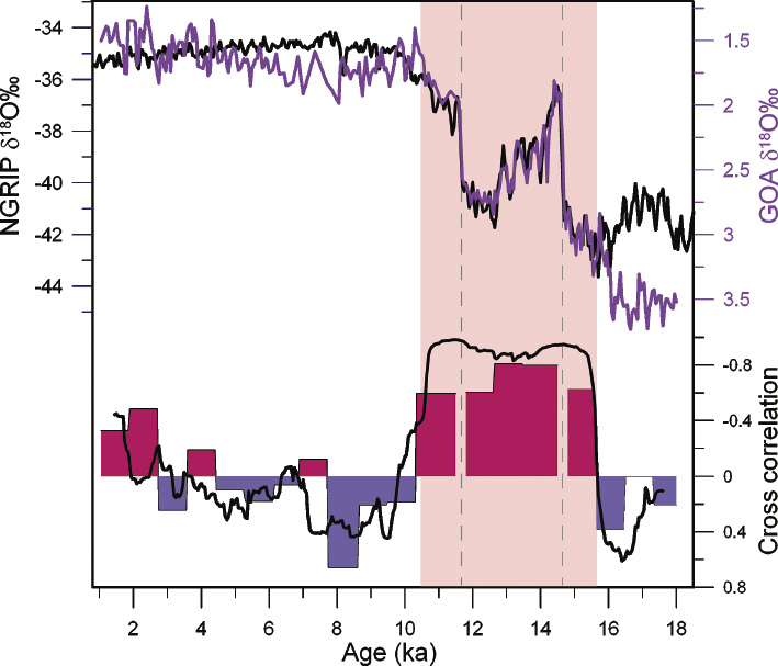
Figure 1: Changes in the correlation between the Greenland NGRIP (Rasmussen et al. 2006) and the Gulf of Alaska (GOA) δ18O records (inverted Y-axis; Praetorius and Mix 2014). Each record is interpolated on a 25 yr time step with a 125 yr Gaussian filter, and the cross correlation is evaluated with both a 2,000 yr centered moving average (black), and in 800 yr stationary windows (red: negative correlation, blue: positive correlation), excluding the 200 years surrounding the abrupt Bølling and Holocene transitions (dashed lines). Both the cross correlation in stationary windows and the moving average indicate a switch from positive to negative correlation (synchronized) prior to the Bølling transition. The interval of high negative correlation is highlighted with pink shading. Negative correlation implies a positive temperature relationship. A center-weighted moving average monitors broad trends in the record by approximating the timing of changes in cross correlation. It is not suited for detecting EWS in isolation of other evaluation as it smooths variance in abrupt transitions. Both the cross correlation in stationary windows and the moving average indicate a switch from positive to negative correlation (synchronized) prior to the Bølling transition.
Although this analysis was based on oxygen isotope data due to its high signal-to-noise ratio, δ18O may be sensitive to temperature, global ice volume changes, and local salinity effects. We have now expanded this work into specific sea-surface temperature proxies (Praetorius et al. 2015), and show that the rapid North Atlantic warming events (as recorded in Greenland) are indeed accompanied by abrupt, high-amplitude warming in the Northeast Pacific, and that abrupt changes in paleo-salinity play only a minor role in the oxygen isotope record. Because these massive warming events are found in the northward advective pathway of waters from lower latitudes, a substantial increase in net northward heat transport is likely. This is somewhat surprising, as the initial warming into the Bølling-Allerød occurred prior to the opening of Bering Strait, during a time when low salinity surface waters would have been trapped in the high North Pacific; radiocarbon evidence suggests that the warming events are not associated with enhanced local overturn (Davies et al. 2014). Coupled global climate models show an amplified surface warming in the North Pacific on centennial time scales in response to increasing radiative forcing due to a shallow mixed layer depth (Long et al. 2014). Such a mechanism may help to explain rapid North Pacific warming in concert with the deglacial rise in atmospheric CO2 concentrations.
Ecological and biogeochemical responses to physical tipping points
Biological and chemical systems may have been entrained in their own dynamics as the deglacial world tipped into warming. For example, it has been known for some time that the oxygen minimum zone expanded abruptly in the North Pacific during both the Bølling-Allerød and early Holocene (Jaccard and Galbraith 2012). These hypoxic events coincided with surface warming (Praetorius et al. 2015), implying strong feedbacks between ocean warming, deoxygenation, and marine productivity, with evidence for tipping-point impacts on the benthic fauna. Abrupt transitions to sedimentary laminations, in close association with enhanced burial of diatom algae, points to a strong role for enhanced sea-surface productivity and subsequent sinking of organic matter in pushing this system across a threshold of hypoxia that was sustained for millennia during each event. Sea-surface warming preceded the increase in productivity and initiation of hypoxia during the Bølling-Allerød transition, suggesting that warming triggered an array of biogeochemical feedbacks in the past, and may imply that future warming could trigger similar feedbacks, leading to more rapid or severe deoxygenation of the North Pacific than what is predicted based on thermal solubility alone.
An abrupt intensification of hypoxia is also observed in the Cariaco Basin in the tropical North Atlantic at similar times to those we observed in the North Pacific (Fig. 2; Gibson and Pederson 2014). The remarkably similar timing and magnitude of sea-surface temperature increase and the near synchronous onset of hypoxia in different oceanic regions in the North Pacific and North Atlantic during the Bølling-Allerød and Holocene transitions, in spite of rather different baseline conditions in the two oceans, imply a prominent role for ocean warming in pushing low-oxygen regions across thresholds of hypoxia. Exactly how the feedback mechanisms work remains poorly known and a subject for future observations and modeling.
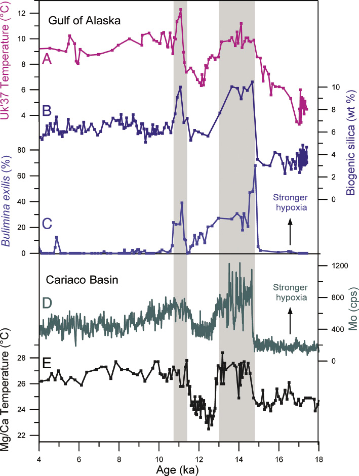
Figure 2: (A) Alkenone (Uk’37)-based sea surface temperature reconstructions from the Gulf of Alaska, North Pacific (Praetorius et al. 2015), with records of (B, C) productivity from the same location and (D) sedimentary redox and (E) temperature from the Cariaco Basin, North Atlantic. (B) Weight percent of biogenic silica (Davies et al. 2011) and (C) abundance of low-oxygen-tolerant benthic species Bulimina exilis (Praetorius et al. 2015). (D) Scanning-XRF record of Mo from the Cariaco Basin (Gibson and Pederson 2014), and (E) Mg/Ca paleotemperature reconstruction (Lea et al. 2003). Gray shaded bars reflect the laminated intervals in the Gulf of Alaska, which also correspond to intervals of strong hypoxia in the Cariaco Basin sediments.
Outlook
New high-resolution paleoceanographic records from the subpolar North Pacific document rapid changes during the last deglacial transition similar in timing to those observed in the Greenland ice cores. Rather than deglacial changes in the North Pacific merely reflecting a downstream response to changes in the North Atlantic region, interactions between basins may be a key element in the emergence of abrupt climate transitions in the Northern Hemisphere.
Although changes in inter-ocean coupling may have important consequences for climate, it remains unclear what regulates connectivity between the North Pacific and North Atlantic. This will be a worthy target for future studies. Development of high-fidelity paleoclimate records with precise and accurate chronology is challenging. Nevertheless, assessing the potential for tipping points in the future demands that we understand the dynamics of rapid climate changes and the biogeochemical responses and feedbacks they triggered in the past.
affiliations
1Department of Global Ecology, Carnegie Institution for Science, Stanford, USA
2College of Earth, Ocean, & Atmospheric Sciences, Oregon State University, Corvallis, USA
contact
Summer Praetorius: spraetoriuscarnegiescience.edu
references
Dakos V et al. (2010) Theor Ecol 3: 163-174
Davies M et al. (2011) Paleoceanography 26, doi:10.1029/2010PA002051
Gibson K, Peterson L (2014) Geophys Res Lett 41: 969-975
Hendy I, Kennett J (1999) Geology 27: 291-294
Jaccard S, Galbraith E (2012) Nat Geosci 5: 151-156
Lea D et al. (2003) Science 301: 1361-1364
Lenton TM et al. (2008) PNAS 105: 1786-1793
Lenton TM et al. (2012) Clim Past 8: 1127-1139
Long S-M et al. (2014) J. Clim 27: 285-299
McManus J et al. (2004) Nature 428: 834-837
Praetorius S, Mix A (2014) Science 345: 444-448
Praetorius S et al. (2015) Nature 527: 362-366
Rasmussen S et al. (2006) J Geophys Res 111, doi:10.1029/2005JD006079