PAGES Magazine articles

Owing to their outstanding temporal resolution, ice cores are well-suited to investigate rapid climate transitions during the last glacial period. They show that the climate system underwent dramatic reorganization on annual-to-decadal time scales during the Dansgaard-Oeschger events.

Figure 1: Schematic of the firn column with typical ranges of depth and age. Adapted from Schwander (1996).

Snow falling on the central parts of polar ice sheets is compressed to firn by the weight of the overlaying snow, eventually turning to ice through sintering and recrystallization (Herron and Langway 1980). The isotopic composition of the snow deposited on the surface (a proxy for the local condensation temperature) and impurities (such as aerosols and dust particles) are preserved in this process. In addition, air is trapped in bubbles during the transition from firn to ice, and can be extracted to study, for example, past greenhouse gas concentrations. Accordingly, the top 50-120 m of an ice sheet consists of porous snow and firn, which allows the air to circulate between the surface and the top of the firn column, while diffusive processes dominate further down the firn column (Fig. 1). Once the transformation from firn to ice is completed, the air is trapped in the ice, and the age distribution and composition of the air in the bubbles are no longer changed.

In the firn column, thermal and gravitational diffusion leads to isotopic fractionation. The isotopic composition of the gas trapped in the ice can thus be used as a temperature proxy during fast temperature changes at the surface of an ice sheet, e.g. by analyzing the 15N/14N ratio (δ15N) of nitrogen gas (Huber et al. 2006; Kindler et al. 2014; Severinghaus et al. 1998).

Through the mixing of air in the firn column, the air entrapped in the ice is considerably younger than the surrounding ice matrix (Fig. 1). This age difference is usually denoted as Δage, and is responsible for the uncertainties when investigating the phasing of events during fast climate transitions. Δage depends mainly on snow accumulation and the firn temperature, such that low snow accumulation and low temperatures cause large Δage, and vice versa. Therefore, maximum Δage values are observed in Antarctica e.g. in the Vostok ice core during the Last Glacial Maximum about 20’000 years ago (Δage of approx. 5000 years), while in Greenland Δage values are considerably lower (up to 1400 years during the Last Glacial Maximum).

Dansgaard-Oeschger events

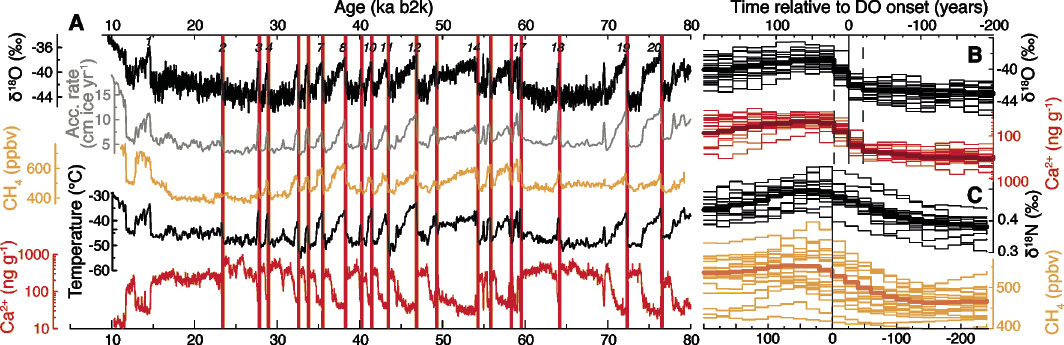
Figure 2: (A) From top to bottom: Glacial NGRIP records of δ18O (Rasmussen et al. 2014), accumulation rate (Kindler et al. 2014), atmospheric CH4 concentration (Baumgartner et al. 2014), δ15N-derived temperature (Kindler et al. 2014), and Ca2+ ice concentrations (Rasmussen et al. 2014). Italic numbers indicate D-O events. Red shades indicate the D-O onsets used in the stack on the right side. All records are plotted on the GICC05modelext age scale (Rasmussen et al. 2014; Seierstad et al. 2014). (B) Stacks of δ18O and Ca2+ at the rapid onsets of D-O events 2-20. A relative time of 0 years corresponds to the onset as defined by Rasmussen et al. (2014), negative time means older ages, positive time means younger ages. (C) Stacks of the rapid D-O onsets of CH4 concentration and δ15N (proxy of temperature change).

During the last glacial period, North Atlantic climate was not stable. The cold stadial periods were interrupted by warmer interstadial periods of durations from 100 to several thousand years. The interstadials, also called Dansgaard-Oeschger (D-O) events, generally show a common shape in time - at the beginning, temperature increases rapidly, and subsequently decreases first slowly, then abruptly to reach stadial values again (Fig. 2a). Other climate parameters mimic this pattern. This Northern Hemisphere temperature pattern is linked to Antarctic temperature by means of the bipolar seesaw (Stocker and Johnsen 2003). This concept proposes that a reduced Atlantic Meridional Overturning Circulation (AMOC) leads to heat accumulation in the southern hemisphere (Southern Ocean) until temperature increases rapidly in the north, whereafter temperature decreases again in the south (EPICA Community Members 2006).

Due to their outstanding temporal resolution and well-constrained chronologies throughout the entire last glacial period, Greenland ice-core records are perfectly suited to investigate fast climate variations in the North Atlantic region (e.g. Huber et al. 2006; Steffensen et al. 2008), while CH4 synchronized Antarctic ice cores can be used to reconstruct mechanisms which link both hemispheres during past abrupt climate changes through the bipolar seesaw (EPICA Community Members 2006).

Duration and rates of change during D-O onsets

In Figure 2b, we stack δ18O and Ca2+ at the onsets of D-O events 2-20. It is evident that the changes in δ18O and Ca2+ are equally abrupt between stadials and interstadials. The transition from stadial to interstadial conditions of δ18O takes place within 1-2 steps of the 20-years-resolution record. Within the data resolution, no significant lead or lag of Ca2+ relative to δ18O can be observed. The mean duration of the climate transition for Ca2+ is also in the order of 40 years. Within these four decades, Ca2+ concentrations decrease by one order of magnitude, and δ18O increases by 3.8‰ on average.

The Ca2+ record is primarily reflecting changes in dust source conditions, most likely from Central Asian desert regions (Biscaye et al. 1997; Svensson et al. 2000), and transport effects. Thus, changes in Ca2+ concentration indicate reorganizations of wind fields and atmospheric circulation patterns at regional to hemispherical scale. The close relative timing of δ18O and Ca2+ changes indicates that the rapid changes in Greenland atmospheric dust loading and in δ18O may be linked to the same large-scale circulation changes.

Gas concentrations stored in ice cores change more slowly than δ18O and Ca2+ because they are well mixed in the atmosphere and have residence times of a decade (CH4) or more (e.g. CO2 and N2O). Due to gas diffusion in the firn column and the slow bubble enclosure process, fast changes of atmospheric gas concentrations are further smoothed in ice cores (Fig. 2c). Huber et al. (2006) calculated an average duration of δ15N increase of 225±50 years for D-O events 9-17. δ15N is controlled by the width in the age distribution of the air enclosed in the ice and by the slow heat conductance in the firn column, which gets rid of the thermal diffusion signal. From the stack of D-O 2-20, we calculate a mean temperature jump of 10.1°C, and a mean CH4 concentration increase of 70 ppb (Fig. 2c). The increase of atmospheric CH4 concentration at the onset of a D-O event shows a slight lag of approximately 50 years, relative to the temperature increase recorded in δ15N in line with the findings of Huber et al. (2006). A direct comparison of gas parameters and ice parameters is difficult, because Δage uncertainty (50-100 years) is comparable to the observed differences of the start of the increase.

The durations of the fast D-O onsets discussed above can be translated into rates of change in CH4 concentrations and temperature. If we assume that δ18O documents the temporal change in surface temperature at the ice-core site (approx. 40 years; e.g. Steffensen et al. 2008) and take the δ15N-derived average temperature increase of 10.1°C, this results in an average temperature increase of 2.5°C/decade. Fig. 2c shows that the increase of CH4 is slightly faster than δ15N. Assuming a rise time of atmospheric CH4 concentration of about 30 years and an increase of 70 ppb, this results in an average rate of change of 23 ppb/decade, however, delayed by a few decades relative to the temperature increase. Comparing these values with modern rates of change (temperature: 0.15°C/decade (global) and 0.46°C/decade (Arctic), last 40 years; CH4: 48 ppb/decade, last 30 years) shows that Greenland temperature increased considerably faster at the onsets of D-O events than modern temperature does, but modern atmospheric CH4 concentration is increasing substantially faster than it did during D-O events. This stresses the strength of the anthropogenic CH4 perturbation in recent decades compared to the most severe natural CH4 changes, and at the same time illustrates how fast earth climate system variations can occur under glacial boundary conditions.

affiliations

1Physics Institute and Oeschger Centre for Climate Change Research, University of Bern, Switzerland

2Niels Bohr Institute, University of Copenhagen, Denmark

3INSTAAR, University of Colorado, Boulder, USA

contact

Simon Schüpbach: schuepbachclimate.unibe.ch

references

Baumgartner M et al. (2014) Clim Past 10: 903-920

Biscaye PE et al. (1997) J Geophys Res 102: 26765-26781

EPICA Community Members (2006) Nature 444: 195-198

Herron MM, Langway CC Jr. (1980) J Glaciol 25: 373-385

Huber C et al. (2006) Earth Planet Sc Lett 243: 504-519

Kindler P et al. (2014) Clim Past 10: 887-902

Rasmussen SO et al. (2014) Quat Sci Rev 106: 14-28

Schwander J (1996) NATO ASI Series I 43: 527-540

Seierstad IK et al. (2014) Quat Sci Rev 106: 29-46

Severinghaus JP et al. (1998) Nature 391: 141-146

Steffensen JP et al. (2008) Science 321: 680-684

Stocker TF, Johnsen SJ (2003) Paleoceanography 18, doi:10.1029/2003PA000920

Svensson A et al. (2000) J Geophys Res 105: 4637-4656

Ocean circulation within the Atlantic is capable of changing rapidly, with important consequences for global climate. Evidence from various climate archives suggests that abrupt transitions in the past were preceded by systematic behavior that could have provided early warning indicators.

The Atlantic Meridional Overturning Circulation (AMOC) redistributes heat, salt and carbon as part of the global thermohaline circulation. Major changes of the AMOC would have global impacts and, as a potential tipping element (Lenton et al. 2008), it is a focus for future projections. The IPCC (2013) concluded that it is very unlikely that an abrupt transition or collapse of the AMOC will occur during the next century for the scenarios considered. However, it is not clear that, under realistic forcing conditions, the complex models used for future climate scenarios are capable of producing the abrupt changes that occurred relatively frequently during the last glacial period (Valdes 2011).

Paleo evidence for abrupt change

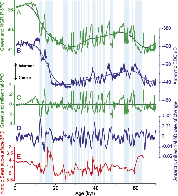
Figure 1: Abrupt climate change over the past 70 kyr. The blue bars indicate stadial events. (A) Greenland temperature proxy record showing the abrupt D-O transitions (NGRIP members 2004). Orbital component is a 7 kyr running mean. (B) Antarctic temperature proxy record showing a more gradual behavior (Jouzel et al. 2007). (C) Millennial-scale component of Greenland temperature. (D) Rate of change of Antarctic temperature showing systematic warming during Greenland stadials and cooling during interstadials (Barker et al. 2011). (E) Proxy record showing sub-surface warming in the North East Atlantic during stadial events (Ezat et al. 2014).

Temperature records obtained from Greenland ice cores provided the first convincing evidence of past abrupt climate change (Fig. 1). The Greenland records revealed repeated transitions (the so-called Dansgaard-Oeschger, D-O, oscillations) between cold, stadial conditions and warmer interstadial conditions, with extremely fast (decades or less) shifts between these states (NGRIP members 2004). These alternations are one expression of a global system, capable of driving major changes in components ranging from ocean temperatures to monsoon rainfall. Massive ice-rafting events across the North Atlantic (Heinrich Events, HE) during some stadial phases (HS events) were associated with particularly cold conditions across the North Atlantic (Shackleton et al. 2000) and suggest the existence of three distinct climate “states” during glacial times.

The ocean’s role in rapid climate change

It has long been argued that D-O and Heinrich variability involved changes in the AMOC and many attempts have been made to test this using paleodata. On a basin scale, water mass tracers, such as benthic foraminiferal δ13C and Cd/Ca ratios and seawater Nd isotopes, suggest a reduction in the ratio of northern versus southern deep water end-members in the Atlantic during northern cold events, particularly those associated with H-Events (Shackleton et al. 2000). On a regional scale, variations in the transport of North Atlantic Deep Water have been reconstructed using a variety of methods including sediment composition, grain size and magnetic analysis (Kissel et al. 2008). These studies suggest a systematic link between high-latitude climate change and variations in deep ocean circulation, even for non-Heinrich stadial events. They suggest a reduction in the deep overflows emanating from the Nordic Seas during cold events, implying a decrease in the production of deep waters through open ocean convection north of Scotland. Concomitant variations in wintertime sea-ice cover across the Nordic Seas have been proposed as an effective means of explaining the very large changes in temperature observed across Greenland associated with D-O transitions (Li et al. 2010).

The AMOC as a tipping element

The magnitude and speed of D-O transitions qualifies as abrupt climate change, yet the nature of the transitions and whether they are “predictable” in some way is debated. Abrupt transitions could be the result of a gradual change in forcing applied to a system containing a threshold (tipping point) or of a large and abrupt change in forcing applied to a system with or without a threshold. In the former case, we could expect “early warning” indicators of the abrupt change as a result of “critical slowing down” as the threshold is approached. A decrease in system resilience close to the bifurcation point would be reflected by an increase in variance and autocorrelation that could be detected given a well-resolved time series of a relevant system parameter. No early warning would be expected for a system without a threshold, or in a system forced through a threshold by a large and rapid change in forcing.

Statistical studies using the Greenland temperature records have produced contrasting results, with early warning being undetected (Ditlevsen and Johnsen 2010) or weakly present (Cimatoribus et al. 2013). Yet there are other reasons to suspect that D-O transitions are the result of gradual forcing through a critical threshold and are not merely stochastic in nature.

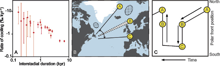
Figure 2: Gradual cooling during an interstadial precedes the abrupt transition to stadial conditions. (A) The rate of cooling (defined here as the rate of change in δ18O) during a Greenland interstadial is related to its duration. (B) Cartoon showing the approximate migration path of the North Atlantic polar front associated with D-O transitions. Stippled areas show approximate locations of modern deep convection. Position A represents interstadial conditions with convection north of Scotland. Stadial conditions are represented by point C with deep convection restricted to south of Iceland. (C) Temporal evolution of the polar front position across a D-O oscillation. From point A, gradual cooling pushes the polar front southwards. On reaching threshold point B, an abrupt southward migration of the polar front occurs with the transition to stadial conditions (point C). It can be seen that a faster rate of cooling between A and B would result in a shorter interstadial. The return to warm conditions is essentially synchronous across the North Atlantic. Modified after Barker et al. (2015).

The abrupt transitions from interstadial to stadial conditions over Greenland are preceded by gradual cooling during interstadial times (Figs. 1,2). Barker et al. 2015 have argued that this cooling is related to a gradual southward migration of the North Atlantic polar front, giving rise to a diachronous transition to polar conditions across the North Atlantic, and leading to an abrupt descent into stadial conditions once a threshold is crossed (Fig. 2b,c). Such a threshold is also implied by the Greenland temperature records themselves, which reveal an inverse relationship between the rate of cooling within an interstadial and the duration of that event (Fig. 2a).

The abrupt transitions from stadial to interstadial conditions, as recorded by the Greenland temperature records, reveal no systematic behavior prior to these transitions. However, using the Greenland temperature records, one cannot differentiate between HS events and non-H stadials even though North Atlantic records suggest much colder conditions during HS events (Shackleton et al. 2000). This can be explained by the insulating effect of sea-ice across the Nordic Seas but implies that the Greenland temperature records are not optimally suited for detecting early indications of impeding interstadial transitions. In contrast, the Antarctic ice core records suggest a continuous build-up of heat across the Southern Ocean throughout all stadial events (Jouzel et al. 2007; Fig. 1d). Moreover, the “Antarctic signal” is not restricted to the remote Southern Hemisphere but can be detected around the Earth as a globally pervasive signal (Barker and Knorr 2007). Furthermore, gradual global warming (that could be the incidental by-product of stadial conditions; Fig. 1) could itself lead to an abrupt strengthening of the AMOC beyond some threshold (Knorr and Lohmann 2007), suggesting that early warning of abrupt warming transitions may be detectable given the right record.

Prone to instability

The ubiquitous cooling observed throughout interstadial periods, leading ultimately to an abrupt transition to stadial conditions (Barker et al. 2015), suggests that whether or not the interstadial mode of AMOC is dynamically stable, its very existence necessitates a transition back to a stadial mode. Equally, if the build-up of heat during stadial conditions (Jouzel et al. 2007; Ezat et al. 2014) is the ultimate cause of an abrupt switch back to interstadial conditions, it could be argued that neither state is truly stable. Thus, the D-O oscillations may be an inevitable consequence of glacial climate, rather than the consequence of random external perturbations. Indeed, the Antarctic temperature record documents the continuous redistribution of heat throughout stadial and interstadial periods alike (Jouzel et al. 2007; Barker et al. 2011; Fig. 1). According to this metric, the AMOC only ever experiences quasi-equilibrium during full interglacial and full glacial conditions (Barker et al. 2011). Thus from a paleo perspective it appears that abrupt transitions in the AMOC can occur in response to gradual change, even if that change is a product of the AMOC state itself. State-of-the-art climate models should be tested to reproduce this sensitivity to learn more about abrupt climate transitions in the past and place more robust constraints on future predictions of AMOC stability.

affiliations

1School of Earth and Ocean Sciences, Cardiff University, UK

2Alfred Wegener Institute, Bremerhaven, Germany

contact

Stephen Barker: BarkerS3cardiff.ac.uk

references

Barker S et al. (2015) Nature 520: 333-336

Barker S, Knorr G (2007) PNAS 104: 17278-17282

Barker S et al. (2011) Science 334: 347-351

Cimatoribus A et al. (2013) Clim Past 9: 323-333

Ditlevsen PD, Johnsen SJ (2010) Geophys Res Lett 37, doi: 10.1029/2010GL044486

Ezat MM et al. (2014) Geology, doi:10.1130/G35579.1

IPCC (2013) Climate Change 2013: The Physical Science Basis. Cambridge University Press, 1552 pp

Jouzel J et al. (2007) Science 317: 793-796

Kissel C et al. (2008) Paleoceanography 23, doi:10.1029/2008PA001624

Knorr G, Lohmann G (2007) Geochem Geophys Geosyst 8, doi:10.1029/2007GC001604

Lenton TM et al. (2008) PNAS 105: 1786-1793

Li C et al. (2010) J Clim 23: 5457-5475

NGRIP members (2004) Nature 431: 147-151

Shackleton NJ et al. (2000) Paleoceanography 15: 565-569

Valdes P (2011) Nature Geosci 4: 414-416

Tipping points are large and potentially irreversible changes in a system. They have been extensively studied in lake ecosystems. This article describes how we can identify past and predict future tipping points and their impacts for lake management.

Lake ecosystems are changing rapidly under growing anthropogenic pressure, with many moving from one functioning state to another across poorly understood thresholds. These changes can be termed regime shifts, which we define as any substantial reorganization of a complex system with prolonged consequences. The cusp between states can be represented as a tipping point or critical transition, where a small perturbation may be sufficient to move the system from one state to another.

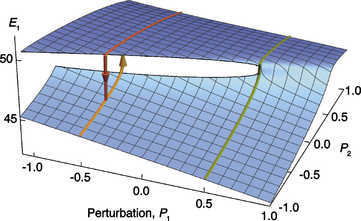
Figure 1: A simple model of a bi-stable system (Weaver and Dyke 2016). The diagram shows how the magnitude of perturbations (P1 and P2) acting on an environmental variable (E1) can lead to smooth, easy to reverse changes in the value of E1 (yellow line) or abrupt critical transitions with hysteresis loops (orange and red lines).

These abrupt, discontinuous changes feature internal processes and feedback loops which reinforce the new state, as in a fold bifurcation (Fig. 1). Consequently, being able to warn of an approaching tipping point before it is reached may allow for policies to be put in place in time.

Lake systems can be complex. But if we assume that the system can occupy more than one stable state, for example oligotrophic “clear water” or eutrophic “turbid water”, then we can formulate simple mathematical models of how different drivers, such as nutrient loading or water-level change, cause the system to transition from one state to another. Such an approach is well established and early warning signals (EWS) or impending tipping points have been formulated for a range of natural and social systems (Scheffer 2009). Much of the original evidence and theory for tipping points and EWS has come from analyses and models of lake ecosystems, but more recently there has been a focus on the analysis of lake sediments (e.g. Wang et al. 2012).

As a lake ecosystem approaches a tipping point, it loses resilience. Models and laboratory experiments suggest that in this condition an ecosystem takes more time to recover from perturbations, a phenomenon known as critical slowing down (CSD). CSD is more likely a source of EWS in systems where the external impacts are relatively small. Where the impacts are large, the lake may flip temporarily in and out of an alternate state, before ultimately settling in the alternative state – a phenomenon known as flickering. In lake ecosystems where external drivers constitute high levels of noise, flickering is a more likely source of EWS than CSD (Scheffer et al. 2012).

While the formulation of EWS is mathematically straightforward, there are a number of challenges in observing them in a real world context. For example, EWS require analysis of the rates of change of certain variables. This requires measurements taken over short intervals from long and highly resolved datasets that are sometimes not available. Furthermore, some studies have shown that regime shifts can arrive without warning (Hastings and Wysham 2010) and that EWS can arise as false positives in any model regardless of critical transitions (Kéfi et al. 2013). Additionally, many mathematical models used to define complex dynamics are low-dimensional simplifications of reality, which risk omitting the very complexity that characterizes the real-world systems. Research priorities include observing or reconstructing EWS signals in time series from real-world lake systems so that relevant theories may be tested and the underlying mechanisms explored.

Empirical examples

Previous research shows that over the past 150 years many lakes have experienced regime shifts in their ecosystems through the effects of atmospheric pollution (acid rain from coal and oil fired power stations) or farming in the drainage basins (nutrient runoff from fertilizer applications) on water quality, and while some have since recovered to their former conditions many have not (Battarbee et al. 2014). While many studies have been undertaken on lake ecosystems in an attempt to identify transitions in state, relatively few have focused on detailed assessments of changes in resilience prior to transition, or attempted to identify EWS prior to a tipping point. Indeed, identifying characteristics of a tipping point, as opposed to more gradual shifts, remains a challenge for lake ecosystem research.

Shallow lake eutrophication typically results in a transition from benthic to pelagic community dominance that may or may not result in an overall shift in algal production. The drivers may be either top-down, such as significant changes in fish populations, or bottom-up through enhanced nutrient loading, or a combination of both. Evidence from temperate studies suggest that changes from clear water plant-dominated systems to turbid, eutrophic systems take 10-100s of years (Sayer et al. 2010). These changes could be interpreted as flickering between states, as the resilience drops and positive feedback loops strengthen. The final stage of settling into the alternative state would be an abrupt transition but further research is required to test these ideas.

Deeper lakes that stratify can also react to change through top-down or bottom-up processes. Some modeling work on instrumental and paleolimnological data has suggested that deep stratified systems do show nonlinear transitions between alternate attractors (Seekell et al. 2013). Other experiments on test lakes (with controls) in Michigan have manipulated the food web over a four-year period by steadily increasing the top predators to the ecosystem to turn the lake from turbid to clear water. All directly measured variables on the manipulated lake showed changes in variability (EWS) a year prior to the completion of the transition (Carpenter et al. 2011; Seekell et al. 2012). The tipping point appears to happen much faster than in shallow lakes, likely due to the speed and magnitude of the drivers (annual vs multi-decadal timescales). Can these effects be upscaled to a whole ecosystem? Batt et al. (2013) compared ecosystem productivity against measured drivers for the same manipulated and control lakes. They found no changes in variance, a typical EWS identified in modeling experiments, but they did define a “first day of alarm” that signifies an up-and-coming tipping point.

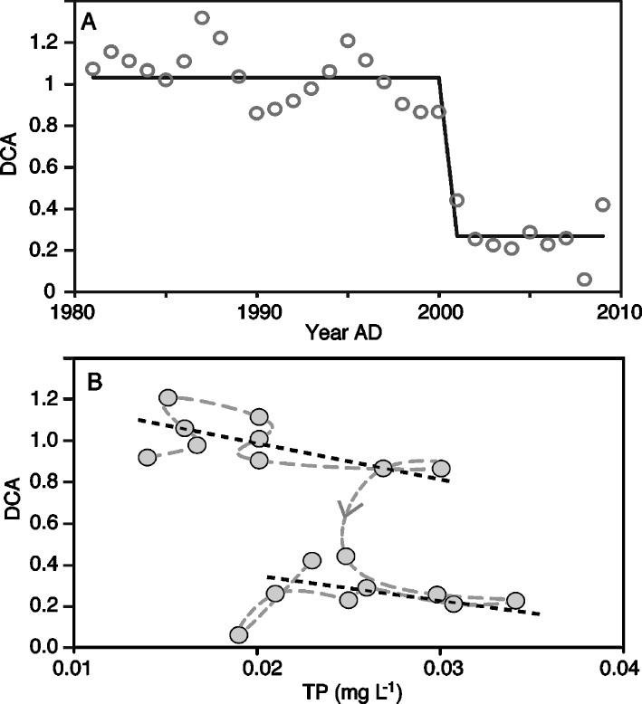
Figure 2: Regime shift, tipping point and alternative stable states at Erhai lake, Yunnan, China (after Wang et al. 2012). (A) Student’s t-test on sequential analyses of diatom DCA data from deep water sediments which indicates a clear tipping point in 2001 from mesotrophic to hypereutrophic states. (B) Phase-space plot of instrumental measurements of total phosphorus (TP) from 1992-2009 plotted against changes in diatom state response (DCA axis 1 scores). The plot shows the two alternative states, the upper state (1992-2001) and lower state (2001-2009) occurred across TP values 0.02-0.03 mgl-1, which is equivalent to 50% of the whole TP scale: this finding is strong evidence for alternative states and hysteresis.

Other work on deeper lakes has focused on how increased nutrient loading can enhance internal nutrient recycling in a positive feedback cycle through hypolimnetic oxygen depletion. At Erhai Lake, China, diatom data showed a significant tipping point in 2001 using both equal and non-equal increment sediment samples. Monitored water quality and algal data before and after 2001 allowed reconstruction of the two stable states and the hysteresis effect predicted by bifurcation theory (Fig. 2). Time series analyses of sediment data suggested the presence of EWS in the form of increased variance a few decades before the transition (Wang et al. 2012; Doncaster et al., in press).

Future challenges

We do not yet understand why tipping points occur in some lakes and not others, nor are we able to identify EWS with confidence. There is much scope for more empirical data collection and analyses targeted at the detection of tipping points and EWS in lake ecosystems. More data will improve our modeling approaches and advance theoretical developments. Paleolimnological data offer great potential in these respects especially where time-series of sub-decadal ecological processes can be resolved at equal increments. Significant advances in identifying and anticipating tipping points in lakes and other systems are not only possible but eagerly awaited by the wide scientific community.

affiliations

1Geography & Environment, University of Southampton, UK

2Nanjing Institute of Geography and Limnology, Chinese Academy of Sciences, Nanjing, China

contact

Peter G. Langdon: P.G.Langdonsoton.ac.uk

references

Batt RD et al. (2013) PNAS 110: 17398-17403

Battarbee RW et al. (2014) Ecol Indic 37: 365-380

Carpenter SR et al. (2011) Science 332: 1079-1982

Doncaster CP et al. (in press) Ecology, doi: 10.1002/ecy.1558

Hastings A, Wysham D (2010) Ecol Lett 13: 464-472

Kéfi S et al. (2013) Oikos 122: 641-648

Sayer CD et al. (2010) Freshwater Biol 55: 500-513

Scheffer M (2009) Critical Transitions in Nature and Society. Princeton University Press, 400 pp

Scheffer M et al. (2012) Science 338: 344-348

Seekell DA et al. (2012) Ecosystems 15: 741-747

Seekell DA et al. (2013) Theor Ecol 6: 385-394

Wang R et al. (2012) Nature 492: 419-422

Weaver IS, Dyke JG (2016) Earth Syst Dyn Discuss doi:10.5194/esdd-6-2507-2015

The PAGES Asia2k summer temperature reconstruction since 800 CE is providing valuable insights into Japanese history. We demonstrate that multi-decadal temperature variability is closely associated with famines and warfare in Japan, resulting in significant societal changes.

Japanese historians have frequently remarked that climate may have had a significant impact on historical events, but have not reached a consensus on the mechanisms of change. A major challenge has been the use of different paleoclimate data based on a range of natural proxies, which were sometimes incorrect or contradictory to one another. In many instances, time series of past climate were arbitrarily selected by historians to support specific arguments. Of particular concern has been the inclusion and recognition of low-quality paleoclimate data for the robust analysis of climate and history relationships in Japan.

The Asia2k reconstruction

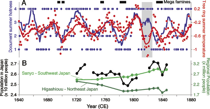
Figure 1: (A) Tree-ring based East Asia summer temperature reconstruction (red; Cook et al. 2013) and document-based Japanese summer hotness estimation (blue; Maejima and Tagami 1986) during 17-19th centuries. Solid circles and thick curves show annual and 11 years running mean values, respectively. Except for the extremely cold winter of 1820 CE (gray shade), both time-series parallel one another closely. Upper black thick lines indicate occurrence of mega famines in northeast Japan. (B) Populations in Japan (black solid) and two regions (green).

The PAGES 2k Network has successfully reconstructed annual changes in continental temperature by integrating many climate-sensitive proxy data over the past 2000 years (PAGES 2k consortium 2013). The strategy to use available datasets with strict selection criteria has helped make more reliable reconstructions. As part of this effort, the Asia2k Working Group has compiled more than 200 tree-ring chronologies beginning before 1600 CE over a wide region in Asia (east of 70˚E), enabling the development of yearly summer temperature variations in individual grid points since 800 CE. Crucially, an average East Asia summer temperature reconstruction has been generated across all 2° grid points north of 23˚N (Cook et al. 2013). Although the original tree-ring chronologies are mainly distributed in inland cold regions, such as Tibet, Himalaya and Mongol, the reconstructed temperature variation corresponds well to the summer temperature index during early modern Japan (Fig. 1A) estimated from documentary records of climate disasters (Maejima and Tagami 1986). Because tree-ring based temperature reconstructions have typically been limited to the last 500 years in Japan, the new Asia2k paleo-temperature data enables us, for the first time, to elucidate climate and history relationships at annual time scales for medieval and ancient Japan before 1500 CE.

Apparent coincidence to Japanese history

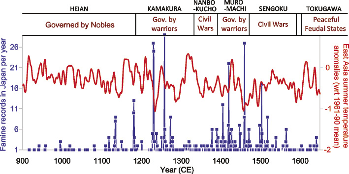
Figure 2: Number of documentary records of famine per year in Japan (blue; Fujiki 2007) and 11-year running mean of East Asia summer temperature (red; Cook et al. 2013). Upper panels define key historic periods (black: name of era; brown: political characteristics).

Multi-decadal variability in the East Asia summer temperature appears to have been enhanced during the 12-15th centuries in medieval Japan, and was associated with numerous famines and wars which culminated in the Sengoku period, characterized by near-constant warring states and societal unrest in the 16th century (Fig. 2). The comparison between temperature and historical events demonstrates that abrupt cooling after 10-20 years of long warmth often caused famines characterized by unprecedented numbers of deaths (Fig. 2) and sustained periods of warfare. Because pre-modern Japanese societies were based on rice paddy cultivation, the increase in rice yields during the warm period might have led to overpopulation, resulting in a society poorly prepared for the following cold period and the inevitable decline in agricultural yields. An example is the Kangi mega-famine in 1230-1231 CE, caused by the abrupt drop in summer temperature after several decades of unprecedented warmth from the middle of the 12th century. Another example is the Kansho famine of 1459-1460 CE, which led to the Onin war (1467-1477 CE), the destruction of the capital city Kyoto, and ultimately led to Japan becoming an aggregate of warring states. Overall, multi-decadal temperature variability from the 12-15th centuries appears to have resulted in many serious societal disturbances, with political government led by nobles during periods of relatively stable climate, followed by civil wars and warrior leadership during subsequent climate instability. It therefore seems that temperature variability was a major driver of societal regime shifts.

The cause-and-effect relationship between multi-decadal climate variability and societal responses can also be observed in the early modern period (17-19th centuries; Fig.1). During the bi-decadal warmth around 1720 and 1800 CE, rice yields rose and population increased even in cold northeast Japan, where rice normally grew poorly under average climate. Local people in northeast Japan became involved in the national rice market, selling excess rice and raising capital to support the finance of local lords and improve the living standard of peasants. These sustained warm conditions thus made adaptation to abrupt cooling difficult, tragically resulting in famines. When the climatic situation changed and famines occurred, the people in Japan started to rebel against the Tokugawa government. Although the Tokugawa government suppressed rebellions at that time, the frequent famines in northeast Japan led to geographical balance change in population and economy (Fig. 1B), leading to a “stronger” southwest region and the reformation of government in 1868 CE conducted by the people from the southwest Japan.

Paleodata for historical studies

The above-mentioned examples for the apparent coincidences between climate changes and historical events in medieval and early modern Japan are, however, special cases. In fact, modes of societal responses to climate change differed depending on the region and period they took place. Abrupt cooling in medieval Japan often caused famines, but we cannot find many indications of famines during the 14th century in historical documents (Fig. 2). While famines directly resulted in war in the late 15th century, they did not cause war in the 13th century. In some feudal domains of northeast Japan during the 18th century, local lords could save people from starving, even when a famine, due to crop failure, killed several hundred thousand people in total over northeast Japan (Fig.1).

As a result, we find there are many lessons embedded in history of societal adaptability to climate change. To date, however, historians have been limited in their ability to critically assess past societal responses to climate changes, because previous studies on human history have not had access to robust paleoclimate data such as that generated by Asia2k. Crucially, we can now learn from past societal struggles to overcome climate disasters by precisely comparing paleoclimate data with the enormous historical and archeological evidence available in Japan. Our results suggest this is a promising way for the promotion of new inter-disciplinary studies between humanity and natural sciences, contributing to the strategy of Future Earth. In Japan, an inter-disciplinary research project “Societal adaptation to climate change: Integrating paleoclimatological data with historical and archaeological evidences” (www.chikyu.ac.jp/rihn_e/project/H-05.html) is now ongoing, to take advantage of the full potential of paleoscience.

affiliations

Research Institute for Humanity and Nature, Kyoto, Japan

contact

Takeshi Nakatsuka: nakatsukachikyu.ac.jp

references

Cook ER et al. (2013) Clim Dyn 41: 2957-2972

Fujiki H (2007) “Chronological Table of Medieval Climate Disaster” (in Japanese)

Maejima I, Tagami Y (1986) Geog Rep Tokyo Metro Univ 21: 157-171

PAGES 2k consortium (2013) Nature Geosc 6: 339-346

The history of the Sahara provides an example for our changing perspective on abrupt change in the Earth system. The emerging concepts can help us to understand past transitions and assess potential future tipping points.

Little does the monotonous and hostile environment of today's Sahara Desert tell us about its colorful past. However, climate and vegetation reconstructions reveal that several thousand years ago, parts of the Sahara resembled a flourishing garden with extensive vegetation and lakes (Jolly et al. 1998). This green Sahara was only the most recent of many green episodes in North Africa's history. The most important driver of these landscape transformations was the permanent change in the Earth's orbital parameters (Kutzbach 1981). When the distance between Earth and Sun is smallest during boreal summer, the larger solar irradiation intensifies the West African monsoon and thus increases rainfall.

Figure 1: Stability landscape of green Sahara and desert. The larger the atmosphere-vegetation feedback, the sharper the transition between the two states. From: Model Calendar 2015, designed by Elsa Wikander at Azote, funded by the Beijer Institute of Ecological Economics and the Stockholm Resilience Centre.

While it is obvious that rainfall is beneficial for vegetation, climate models indicate that vegetation can also enhance rainfall. First, the dark vegetation absorbs more sunlight than the bright desert and provides energy for convection (Charney et al. 1975). Second, the evaporation from vegetation and lake surfaces feeds the water back into the atmosphere (Rachmayani et al. 2015). Vegetation and rainfall are therefore linked in a self-amplifying process, a positive feedback. The stronger this feedback, the more abrupt the transition from a green Sahara to a desert (Fig. 1).

Whereas orbital parameters change gradually over thousands of years, model results (Claussen et al. 1999) and a dust record from the Atlantic (de Menocal et al. 2000) suggested a quite rapid vegetation loss at the end of the green Sahara. This seemed to support the view of a switch from a green state to a desert state, a natural climate catastrophe comparable to a chair suddenly tipping over when it is slowly tilted. Such tipping points have been found not only in atmosphere-vegetation models (Brovkin et al. 1998), but also in simple models representing ocean circulation, Arctic sea ice, ice shields, savannah and lake ecosystems, and the East Asian and Indian monsoons.

Tipping points in a world of complexity

Each tipping point in the simple models mentioned above results from a positive feedback. However, in reality, the rate of a transition is not a question of feedbacks alone. For instance, fast fluctuations in the weather permanently perturb the vegetation and other slow components of the Earth system. These fluctuations thus superimpose an otherwise smooth transition and can either make it more gradual or even more pronounced (Liu et al. 2006).

Figure 2: Idealized abundance of East Saharan plant types from 6000 to 3500 years ago (from left to right) with Acacia (orange), Poaceae (green) and tropical plant taxa (red). Pollen records after Kroepelin et al. (2008), drawing by Dominique Donoval, Max Planck Institute for Meteorology, Hamburg.

Moreover, there are reasons to believe that the spatial heterogeneity of the land surface tends to make transitions smoother on large spatial scales (Brook et al. 2013). Indeed, different records from the Sahara, such as pollen reconstructions from northern Chad (Kroepelin et al. 2008; Fig. 2), suggest a spatially inhomogeneous transition to today's desert and a gradual decrease in rainfall. Theoretical modeling studies confirm that if different locations are only weakly connected or very dissimilar, every location changes with its own timing, and transitions tend to be gradual on large scales (van Nes and Scheffer 2005). Even in the case of a uniform climate, vegetation still consists of different plant types with different moisture requirements, promoting a gradual change in vegetation composition instead of a singular vegetation dieback (Claussen et al. 2013; Fig. 2).

It is therefore quite clear that the Sahara Desert was not born in one synchronized tipping event. Nonetheless, the case of the green Sahara reminds us that we also need to take spatial interactions into account, because the winds and currents in the atmosphere and ocean couple different locations. Naturally, this connection tends to be strongest between adjacent places since properties like water and energy are transported from one place to the next. But large-scale circulation features like the African monsoon or the ocean's overturning circulation can also couple locations very far from each other. Strong links in the network of interactions can synchronize transitions and promote abrupt change far from the origin of its occurrence. An abrupt climate change at a single location may thus trigger a domino effect of climate changes at different locations. The question is therefore not only whether tipping points exist but also whether there are local hotspots where a system is particularly vulnerable (Bathiany et al. 2013).

Finally, neither climate feedbacks nor spatial interactions are required to obtain abrupt change on a local level. First of all, ecological systems can have tipping points of their own (Scheffer et al. 2001), and many physical and biological systems have intrinsic thresholds, like the freezing temperature of water or the wilting point of plants. Secondly, a shift in the position of sharp spatial gradients or circulation patterns can cause abrupt change at a particular location. For example, the gradual spatial shift of the vegetation distribution may locally be seen as a sudden desertification. Abrupt change in paleorecords like the dust record by de Menocal (2000) could thus be interpreted to result from a shift in the desert boundary or the wind direction.

An uncertain future

In the light of all these mechanisms at play, the reconstructions from the Sahara leave room for interpretation. Has the Sahara taken its green secret to the grave? And are tipping points only a Fata Morgana, caused by oversimplified models? Research on other potential climate tipping points indicates that this may be true. So far, comprehensive climate models cannot convincingly answer the question if large-scale climate tipping points are ahead in the near future (Drijfhout et al. 2015). However, there is evidence that abrupt climate changes happened in the Earth's history. The potential damage such events may cause, and the large uncertainty of their occurrence, require us to assess the risk of future abrupt change by improving our scientific understanding.

The crucial questions of this assessment are the same as for the Sahara. What is the balance of the relevant feedbacks? How homogeneous is the system and are there strong spatial connections? What is the interplay between fast variability and slow system components, and what can we learn from the variability? Are there natural thresholds which promote or prevent abrupt change? As the physical or biological processes differ in each case, answers may depend on which potential tipping point is considered. Bridging the gap between the world of tipping point concepts and the world of process understanding will therefore be key to scientific progress. The green Sahara provides an example for this challenge. Even though its decline was overall more gradual than previously thought, it remains a fruitful case study to explore the above questions. Insofar, the green Sahara has not turned to dust, but flowers in a greater context.

affiliations

1Department of Environmental Sciences, Wageningen University, The Netherlands

2Max-Planck-Institute for Meteorology, Hamburg, Germany

3Meteorological Institute, University of Hamburg, Germany

4Center for Adaptation to a Changing Environment, ETH Zürich, Switzerland

contact

Sebastian Bathiany: sebastian.bathianywur.nl

references

Bathiany S et al. (2013) Earth Syst Dynam 4: 63-78

Brook B et al. (2013) Trends Ecol Evol 28: 396–401

Brovkin V et al. (1998) J Geophys Res 103: 31613-31624

Charney J et al. (1975) Science 187: 434-435

Claussen M et al. (1999) Geophys Res Lett 26: 2037-2040

Claussen M et al. (2013) Nat Geosci 6: 954-958

de Menocal P et al. (2000) Quat Sci Rev 19: 347-361

Drijfhout SS et al. (2015) PNAS 112: 5777-5786

Jolly D et al. (1998) J Biogeog 25: 1007-1027

Kroepelin S et al. (2008) Science 320: 765-768

Kutzbach JE (1981) Science 214: 59-61

Liu Z et al. (2006) Geophys Res Lett 33, doi:10.1029/2006GL028062

Rachmayani R et al. (2015) Clim Past 11: 175-185

Scheffer M et al. (2001) Nature 413: 591-596

van Nes E, Scheffer M (2005) Ecology 86: 1797-1807

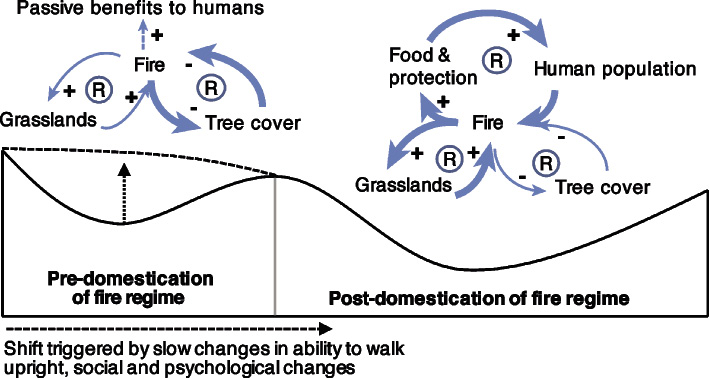
Social-ecological regime shifts involve large, often abrupt, reorganizations in interlinked social and ecological systems. The domestication of fire illustrates how physiological and social changes enabled humans to start actively controlling fire, dramatically reshaping the environment and society itself.

While many changes to the environment occur gradually in response to changing conditions, some changes occur abruptly and may be difficult or impossible to reverse. Examples of such changes have been documented in terrestrial, aquatic, marine and climate science, as well as in archeology and psychology, at timescales ranging from paleo records to contemporary observations (Scheffer 2009; also see www.regimeshifts.org). In this article, we briefly introduce the notion of social-ecological regime shifts, namely abrupt shifts that involve components of both social and ecological systems.

What is a social-ecological regime shift?

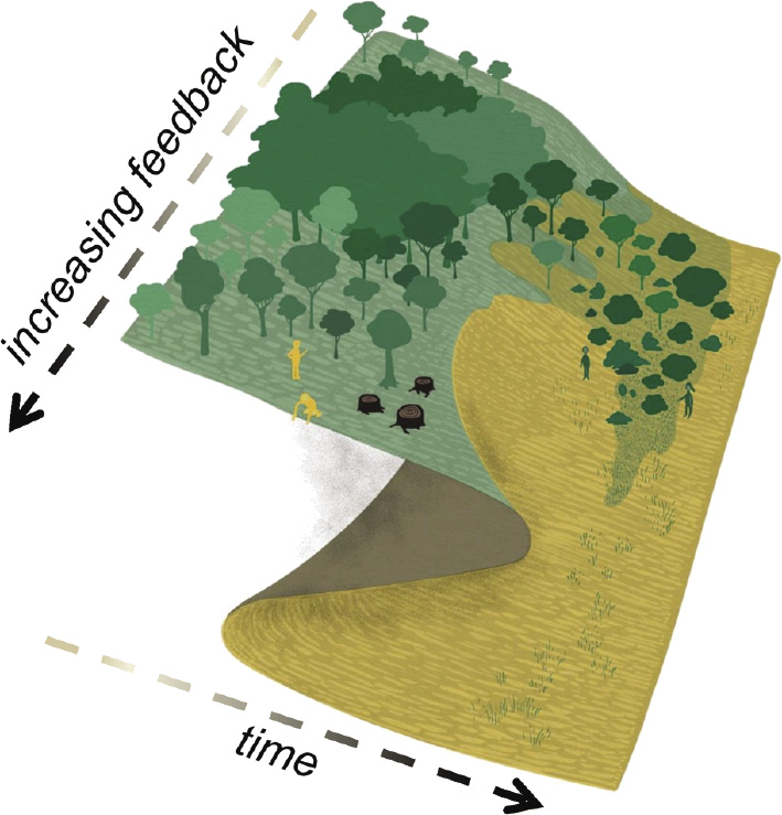
Figure 1: Simplified schematic of the shift in dominant systemic feedback processes associated with the domestication of fire and increased global abundance of grasslands. Bold arrows depict dominant feedbacks shaping social and ecological dynamics in the different regimes; R depicts reinforcing feedbacks.

There is growing interest in social-ecological regime shifts, which we define as a substantive change in the structure and function of interconnected social-ecological systems (SES). Such shifts are associated with a reconfiguration of dominant feedback processes and typically arise from a combination of gradual changes in underlying conditions and a large external shock (Biggs et al. 2012; Fig. 1). Although the shift itself may take decades or centuries, it is usually abrupt relative to the duration of each regime. Social-ecological regime shifts are important as they often have substantive impacts on the ecosystem services and benefits people obtain from SES, and often occur unexpectedly.

While studies have addressed regime shifts in ecological, and to some extent, social systems, there has been limited work on shifts in coupled SES. As with the broader emerging area of SES studies, it is still unclear how social-ecological regime shifts can be most usefully conceptualized and analyzed. Currently, the notion of social-ecological regime shifts can refer to: (1) shifts that arise from ecological dynamics (e.g. eutrophication) and consider the social and economic impacts of these changes; (2) shifts that arise from social dynamics (e.g. introduction of new legislation) and their consequent environmental effects; and (3) cases where the actual shift itself arises from the interaction of social and ecological processes (e.g. harvesting of common pool resources). The latter is perhaps most interesting as it may account for shifts that cannot arise from either social or ecological dynamics, but only occur due to the interaction of these components (Lade et al. 2013).

The concept of social-ecological regime shifts may differ somewhat from that of ecological regime shifts in terms of the type of changes it helps explain. Rather than focusing on the potential for systems to flip “back and forth” between alternate regimes (e.g. clear vs murky water lakes), it may be more useful in explaining “punctuated” change over time – i.e. periods of relatively rapid change that separate longer periods that are relatively stable, but quite different from one another in terms of SES structure and function. The inclusion of social dynamics, which enhances memory, learning, and anticipation in SES, amplifies the role of history and path dependence, reducing the reversibility of shifts. The domestication of fire illustrates this dynamic very clearly.

Domestication of fire as a social-ecological regime shift

Learning how to control fire dramatically changed how humans interacted with each other and their natural environments. Fire domestication appears to have become widespread among hominins by some 300-500 thousand years ago (Sandgathe et al. 2011). Researchers have argued that this marks the start of the Anthropocene and humanity as an Earth-transforming species (Glikson 2013).

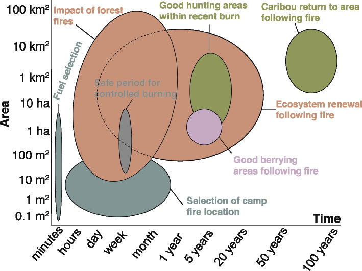
Figure 2: Spatial and temporal dimensions of knowledge related to fire use and its impacts held by Anishinaabe elders in Ontario, Canada, and the areas of expertise they require. Modified from Miller and Davidson-Hunt 2010.

The domestication of fire involved a shift from a long period in which hominins only passively enjoyed the benefits of fire, to a situation where they actively controlled its use (Goudsblom 2015). Researchers believe that active control of fire required physiological changes, in particular the ability to walk upright, which enabled people to use sticks to transport fire and supply it with fuel. However, social and psychological changes were also crucial: obtaining fire from wildfires, and handling and maintaining it required effort, observation, patience, anticipation and social negotiation (Twomey 2013). Before hominins could actively control fire, these social and mental skills had to become part of a learned repertoire of shared ways of thinking and doing (Goudsblom 2015; Sandgathe et al. 2011; Fig. 2).

The domestication of fire changed human demography and social interactions, and fundamentally restructured the ways in which hominins interrelated with their environments. On-site fires in hearths were used to cook food, which greatly expanded the range of foods that hominins could eat and preserve (Wrangham 2009). On-site fires also helped fend off large hominin predators such as saber-toothed cats, drive off mosquitoes and poisonous animals, harden and bend tools, and provide a source of warmth and light. They could also be used for signaling. Off-site burning in the wider landscape similarly helped hominins improve their access to food and make predators more visible. Burning of the landscape was also important for clearing vegetation, driving and attracting animals, clearing pathways, waterholes and campsites, signaling, asserting rights, warfare, ritual activities, and for aesthetic pleasure and entertainment (Scherjon et al. 2015).

Anthropogenic burning of the landscape was typically patchier, and more extensive and intensive than wildfires, and in time reshaped entire ecosystems (Bowman et al. 2011). This impact is most clearly expressed in the increasing global abundance of grasslands after the domestication of fire (Pyne 2013). Control of fire also changed the balance of power between hominins and the species they competed with for food (including other hominin groups), or that preyed on them. Anthropogenic burning of landscapes may have contributed to the mass extinction of large animals during the Pleistocene (Rule et al. 2012). The use of fire therefore radically changed the ecological niche of (early) humans (Odling-Smee et al. 2003).

This example illustrates how ecological, social and psychological changes reinforced one another to produce far-reaching changes, that not only permanently reshaped ecosystems and human society, but also the relationship between humans and nature (Fig. 1). This massive systemic reconfiguration has been argued to have set the stage for further large-scale social-ecological regime shifts. Changes involved in the domestication of fire spurred other social developments such as the creation of language, development of tools, population growth, enculturation (the learning of socially learned habits, routine and norms), and social distinction (Twomey 2013) that created the possibility for further radical innovations in time, most notably the domestication of plants and animals for agriculture (Burton 2009).

Conclusion

Social-ecological regime shifts are important from both a scientific and a policy perspective, as they provide a conceptual framework for understanding non-linear change associated with restructuring of coupled SES. Over shorter time horizons, social-ecological regime shifts often have large impacts on the functioning of ecosystems and society, and therefore on human wellbeing. Furthermore, such shifts usually occur unexpectedly and are often difficult or impossible to reverse, making them difficult for society to cope with or adapt to.

Over longer time horizons, social-ecological regime shifts may have far-reaching effects, fundamentally restructuring the relationships between people and nature and the long term trajectory of global change. The potential for such radical transformative change suggests that, in the context of the tremendous sustainability challenges society faces today, we should consider more deeply how shifts to more sustainable societies could unfold. The diverse, interconnected set of changes involved in the domestication of fire suggests that a transition to more sustainable societies is unlikely to involve only the development of new technologies and legislation that reduces environmental impacts. Instead, such technological and institutional changes are likely to fundamentally reshape both society and the environment in time, and transform the relationship between people and nature in ways that are difficult to foresee.

affiliations

1Stockholm Resilience Centre, Stockholm University, Sweden

2Centre for Complex Systems in Transition, Stellenbosch University, South Africa

contact

Reinette Biggs: oonsie.biggssu.se

references

Biggs R et al. (2012) In: Hastings A, Gross L (Eds) Encyclopedia of Theoretical Ecology. University of California Press, 609-617

Bowman DMJS et al. (2011) J Biogeogr 38: 2223-2236

Burton F (2009) Fire: the spark that ignited human evolution, University of New Mexico Press, 246pp

Glikson A (2013) Anthropocene 3: 89-92

Goudsblom J (2015) Fire and Civilization [In Dutch: Vuur en Beschaving], Van Oorschot, 295pp

Lade S et al. (2013) Theor Ecol 6: 359-372

Miller MA, Davidson-Hunt I (2010) Hum Ecol 38: 401-414

Odling-Smee FJ et al. (2003) Niche construction: the neglected process in evolution, Princeton University Press, 488pp

Pyne S (2013) Fire: Nature and Culture, Reaktion Books, 207pp

Rule S et al. (2012) Science 335: 1483-1486

Sandgathe DM et al. (2011) PNAS 108: E298

Scheffer M (2009) Critical transitions in nature and society, Princeton University Press, 400pp

Scherjon F et al. (2015) Curr Anthropol 56: 299-326

Twomey T (2013) Camb Archaeol J 23: 113-128

Wrangham R (2009) Catching fire: how cooking made us human, Basic Books, 320 pp

Pore moisture within desert sand dunes provides a novel archive for paleomoisture availability. Hydrostratigraphies are produced from variations in chemical tracers in a vertical profile. The applicability has been demonstrated in drylands in five continents and three examples are given here.

Reconstructing past rainfall fluctuations in drylands is challenging. The deposition of sedimentary archives, such as sand dunes, are mediated by a number of factors, of which changing moisture availability is just one. Former river courses, and former lakes fed by rivers, often record changes imported from a climatic zone outside their dryland location (exogenous systems). Speleothems are restricted to limestone terranes and tend to be discontinuous records in drylands. Isotopic records within hyrax middens have growing potential, but are also spatially restricted to areas with rock-ledge habitats. Therefore, developing further proxies capable of recording changes in moisture availability is extremely valuable for dryland Quaternary environmental reconstruction.

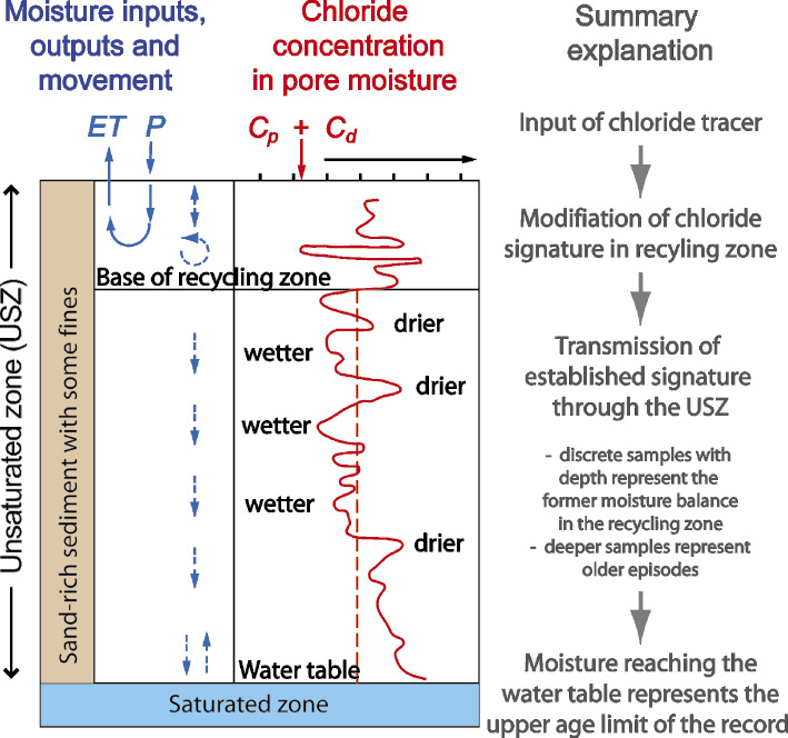
Figure 1: Schematic diagram to demonstrate the basis of the unsaturated zone hydrostratigraphy approach (P is precipitation, ET is evapotranspiration, Cp is concentration of chloride in precipitation and Cd is concentration of chloride in dry deposited material), modified from Stone and Edmunds (2016).

Chemical tracers within sand dune pore moisture offer a novel additional proxy for paleomoisture availability. When and where this moisture moves downward, fluctuations in its chemical signature with depth can be utilized to establish a record of changes to moisture availability through time, based on the transport of a signal built up in the near-surface zone (Fig. 1). The resolution and timescale of the preserved hydrostratigraphy depends on the rate of moisture movement and the thickness of sediment (Stone and Edmunds 2016). Applications over a range of timescales are briefly explored to demonstrate the utility of this approach.

Basis of tracer technique

Pore moisture in sand dunes above the water table is described as the unsaturated zone (USZ) of the hydro(geo)logical cycle. It is in this USZ that hydrostratigraphies can be reconstructed, based upon variations in chloride concentration in pore moisture. The chloride signal is established in the near-surface recycling zone, and this inherited signal is then transmitted vertically in the moisture that is infiltrating through the sediment, so that a depth-based profile of samples represents a temporal record (Fig. 1).

The input of moisture at the surface from precipitation contains solutes, including chloride. The long-term average concentration of this input can be established empirically, and varies between regions as a function of continentality. The chloride input gets modified in the near-surface zone by evapotranspiration, which removes water and enriches the chloride concentration, and by mixing (Fig. 1). Below the zone of recycling, moisture moves downwards, and movement is closest to homogenous in sand-rich sediments containing some finer-fraction sediment (e.g. Gehrels et al. 1998). This means that the concentrations of chloride in pore-moisture at sequential depths are a record of a climatically driven process in the zone of recycling before being transmitted down to that depth. The record can be read as low(high) chloride concentrations recording high(low) moisture availability. A certain degree of smoothing of the record will have occurred in the recycling zone, including smoothing variations between individual rainfall events.

Records of land-use changes and precipitation

USZ hydrostratigraphies can be used to quantify increases in moisture flux through sediments as a result of land-use change. In southwestern Australia, clearance of native eucalyptus vegetation increased recharge rates from ~0.1 mm yr-1 under intact vegetation to 2.5-8.5 mm yr-1 and 3.8-28.0 mm yr-1 under pasture and cereal cropped land respectively (Cook et al. 1994). This is demonstrated clearly in the hydrostratigraphy by a vertical displacement of a single subsurface chloride peak in cleared sites compared to intact sites.

The influence of artificial irrigation can also be investigated. In the Thar Desert, northwest India, multi-decadal length hydrostratigraphies demonstrate a recharge rate under irrigated cropland of 18-98 mm yr-1 as compared to 2.7-5.6 mm yr-1 in a non-irrigated dune (Scanlon et al. 2010).

Over timescales of a few hundred years, the potential of USZ hydrostratigraphies as proxies for precipitation has also been demonstrated. For example, a 108-year-long hydrostratigraphy from Louga, Senegal correlates well with both a local precipitation record and Senegal River flow data, and records the 1970s Sahel drought and the 1940s dry period (Edmunds and Tyler 2002).

Records of climatic change in central Asia

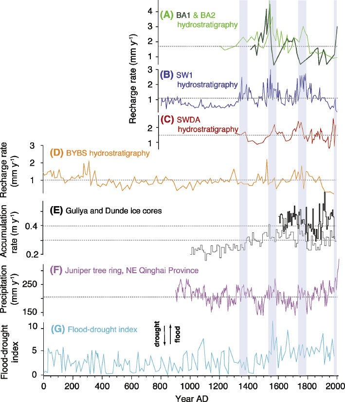
Figure 2: Paleohydrologic records from five USZ hydrostratigraphies from the Badain Jaran desert (A) BA1 (solid line) and BA2 (dashed line) near Baoritelegai (Ma and Edmunds 2006), (B) SW1 near Sayinwusu (Ma and Edmunds 2006), (C) SWDA near Lake Sayinwsus (Gates et al. 2008), (D) BYBS near Lake Bayan Bur (Ma et al. 2009) and (E) Dunde (black line) and Guliya (gray line) ice-core accumulation rate (Thompson et al. 1997), which are ca. 400 km and 2000 km from the Badain Jaran desert. (F) Juniper tree-ring growth record from the NE Qinghai Province, China (Sheppard et al. 2004), which is ca. 500 km south of the Badain Jaran desert. (G) drought-flood index for China from historical documents (Zhang and Crowley 1989), modified from Stone and Edmunds (2016). The blue shaded vertical lines highlight where at least two hydrostratigraphies and two or more of the supporting proxy archive record wetter than average conditions.

Arguably the most significant development for dryland Quaternary environmental reconstruction using this approach comes from the decadal-scale resolution, multi-millennial length hydrostratigraphies from mega-dunes within the Badain Jaran desert in China (e.g. Ma and Edmunds 2006; Gates et al. 2008; Ma et al. 2009). The longest is a 30 m record spanning 2050 years, with four others >500 years. Comparisons with independent paleohydrological proxies for northern China have been made, which highlight wetter intervals in this region around 1350-1400, 1550-1600 and 1750-1800 and after 1990 (Fig. 2A-D). The three earliest wetter intervals are supported by above-average values for precipitation reconstructed from Juniper tree-ring growth records from the northeast Qinghai Province (Sheppard et al. 2004) and the middle phases are also phases of above-average ice-core accumulation in the Guliya ice core (Thompson et al. 1997) and above-average wetness in the flood-drought index (based on historical documents) (Zhang and Crowley 1989). However, the overall correspondence is not perfect, with some larger incursions in the other proxies not appearing in the USZ hydrostratigraphies, suggesting some regional complexity in paleohydrology in this region.

Reconstructing long-term dryland aridification

Initially driven by a motivation to assess whether the deep USZ in the semi-arid western United States might safely store nuclear waste without contaminating groundwater, more than a dozen hydrostratigraphies record an aridity trend through the Late Glacial and into the Holocene (e.g. Scanlon 1991; Phillips 1994; Tyler et al. 1996). The majority of profiles place this shift at around 16,000 to 13,000 years ago. There is one 240 m thick hydrostratigraphy at the Nevada nuclear test core than contains an earlier cycle from higher recharge to greater aridity during Marine Oxygen Isotope Stage (MIS) 5 (Tyler et al. 1996).

Conclusions and outlook

The unsaturated zone (USZ) in dryland environments is a novel and valuable archive, providing a direct paleomoisture proxy, where the enrichment of chloride acts as a tracer for the balance between precipitation and evapotranspiration. The sand-rich sediments required for this approach cover a portion of drylands where it is extremely challenging to reconstruct hydrological variations over the Quaternary, owing to poor preservation of biological material and a scarcity of water-lain sediments and speleothems.

Further development of modeling approaches that incorporate transient fluxes of water and tracer input concentrations (Ginn and Murphy 1997) will continue to reduce uncertainties within USZ hydrostratigraphies. Studies must routinely verify the suitability of the sediment texture at a site-by-site basis and avoid sediments that experience a very heterogeneous vertical flow of water.

USZ hydrostratigraphies have proven potential within drylands (Stone and Edmunds 2016). Depending on the thickness of the USZ sediment and the rate of moisture infiltration, hydrostratigraphies can record low-resolution trends in humidity-aridity over deglacial timescales, a decadal-resolution paleomoisture proxy for the last two millennia or quantify changes in moisture flux in sediment resulting from anthropogenic land use change.

affiliations

1School of Environment Education and Development, The University of Manchester, UK

2School of Geography and the Environment, University of Oxford, UK

contact

Abi Stone: abi.stonemanchester.ac.uk

references

Cook PG et al. (1994) Water Resour Res 30: 1709-1719

Edmunds WM, Tyler SW (2002) Hydrogeol J 10: 216-228

Gates JB et al. (2008) Holocene 18: 1045-1054

Gehrels JC (1998) Hydrolog Sci J 43: 579-594

Ginn TR, Murphy EM (1997) Water Resour Res 33: 2065-2079

Ma J, Edmunds WM (2006) Hydrogeol J 14: 1231-1243

Ma J et al. (2009) Palaeogr Palaeocl 276: 38-46

Phillips FM (1994) Soil Sci Soc Am 58: 15-24

Scanlon BR (1991) J Hydrol 128: 137-156

Scanlon BR et al. (2010) Hydrogeol J 18: 959-972

Sheppard PR et al. (2004) Clim Dyn 23: 869-881

Stone AEC, Edmunds WM (2016) Earth-Sci Rev 157: 121-144

Thompson LG et al. (1997) Science 276: 1821-1825

Tyler SW et al. (1996) Water Resour Res 32: 1481-1499

Zhang P, Crowley TJ (1989) J Clim 2: 833-849

Over the last 20 years, the PAGES-endorsed IMAGES program (International Marine Past Global Change Study, http://www.images-pages.org/) supported 18 sea-going expeditions onboard the 120-meter-long Research Vessel Marion Dufresne. This vessel, operated by the French Paul-Emile Victor Polar Institute, was equipped with an in-house-developed, unique sediment coring facility, called CALYPSO, which allowed for the retrieval of high-quality, long marine cores at sites of high sedimentation rates. The vessel currently holds the world record for the longest marine core ever retrieved - 64.5 m. These cores enabled the comparison of marine and ice-core records at the same resolution for the first time, and tremendously improved the understanding of past oceans dynamics.

Figure 1: Research Vessel Marion Dufresne in dry dock during her complete refit (photo by Damen Shiprepair Dunkerque).

After 20 years of existence, both the coring system and the vessel were upgraded (Fig. 1) in an initiative funded by the French government to provide the scientific community with top-notch technological marine support for the new generation of coring tools. The new coring equipment, developed within the CLIMCOR project (http://climcor-equipex.dt.insu.cnrs.fr/?lang=en), provides the chance to collect high-quality oceanographical data as crucial complements for paleoclimatic data.

The objective is to routinely retrieve 75-meter-long, undisturbed sediment cores in any water depths to adequately address the scientific targets highlighted by international scientific programs. To achieve this, a specially designed DYNEEMA synthetic cable, with controlled minimum elasticity, has been developed to drastically reduce the sediment disturbance upon coring of the top meters of the core, which was the main flaw of the previous coring system. The first sea trials, operated in November 2015, show that when the corer is triggered just above the seabed at a water depth of 4500 m, the elastic rebound of the cable has been strongly reduced from 16 to 9 meters. This elastic rebound is due to the sudden release of the corer weight that was set to five tons for this test. This minimized elastic rebound should now guarantee undisturbed sediment recovery down to 4000 m water depth.

Other technical improvements lead to better control of the operation with a suite of pressure and acceleration sensors on the corer head and the triggering system, and software (e.g. CINEMA software developed by Ifremer; Bourillet et al. 2007; Woerther et al. 2012), allowing a detailed monitoring of the coring operation, increased safety of the operation both for the personnel and instrumentation, an optimization of ship time, and a larger choice of environment-data collection during the coring process, including detailed information on the degree of preservation of the recovered sediment sequence.

During its midlife refit, the vessel was adapted to suit this new long-core challenge. Scientific deck equipment, such as the coring winch and associated frame, the hydrological winch and the deployment system were upgraded. The coring handling equipment capacity was increased to 45 tons SWL (Safe Working Load) and the ship bulwark was modified to allow easier and safer deployment of a 75-meter-long corer.

Finally, a new suite of acoustic sensors was integrated on board the vessel, including KONSBERG EM122 and EM710 multibeam echo-sounders and a SBP 120-3 sub-bottom profiler. This equipment provides the highest image quality of the seabed and upper sediment, allowing an accurate survey of the coring targets. A new Ultra Short Base Line system (USBL Posidonia) was integrated to accurately locate the various corers on the seabed.

Due to the massive investment through the ”Investissements d'Avenir” French national program, the refitted Marion Dufresne offers brand new and top-class coring equipment, able to collect up to 75-meter-long continuous sequences of undisturbed sediments at water depths as deep as 4500 m, which is available to the international paleoceanographic and paleoclimate communities for upcoming exciting and stimulating expeditions.

affiliationS

1Ecole Normale Supérieure, LMD, Paris, France

2French Polar Institute Paul Emile Victor, Plouzané, France

3CNRS, National Institute for Earth Sciences and Astronomy, Paris, France

4Bordeaux University, EPOC, Pessac, France

contact

Denis-Didier Rousseau: denis.rousseaulmd.ens.fr

Links

http://climcor-equipex.dt.insu.cnrs.fr/

http://www.cnrs.fr/

http://www.institut-polaire.fr/

http://www.agence-nationale-recherche.fr/investissements-d-avenir/

references

Bourillet J-F et al. (2007) 6th International Conference on Offshore Site Investigation and Geotechnics: Confronting New Challenges and Sharing Knowledge. Society of Underwater Technology, London, UK

Woerther P et al. (2012) Improving in piston coring quality with acceleration and pressure measurements and new insights on quality of the recovery, INMARTECH 2012, Texel, the Netherlands

The MD203 ACCLIMATE expedition was the first coring cruise onboard the Research Vessel Marion Dufresne since her midlife refit in 2015 (Rousseau et al. 2016). Taking place in March 2016 in the South Atlantic Roaring Forties and Howling Fifties, this cruise provided a full-scale exercise to test, in rough sea conditions, the latest generation of sediment coring equipment.

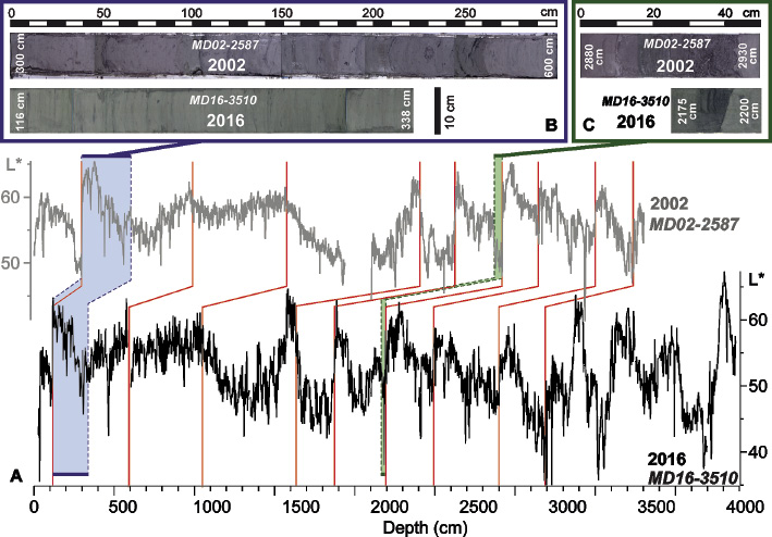
Figure 1: Comparison of cores MD02-2587 (35°17.7’S, 29°22.2’E, 4468 m) and MD16-3510 (35°21.38’S, 29°14.78’E, 4435 m) collected in 2002 and 2016, respectively, at the same South African margin site. (A) Downcore reflectance (L*) changes in both cores on their respective depth-scales. Red lines highlight conspicuous color changes synchronous in both cores. The 2002 core is stretched compared to the 2016 core. (B) Core photographs of the same time period (blue area) covered by 300 and 222 cm of sediments in the 2002 and 2016 cores, respectively. Dark layers are straight in the 2016 core, while bent in the 2012 core. (C) Core photographs of the same turbiditic event (green area). The characteristic downward coarsening of turbiditic sediments is stretched in the 2002 core. These features illustrate the absence of sediment stretching and deformation in the 2016 core, in opposition to the 2002 core.

To illustrate the unprecedented quality of long sediment sequences taken with the improved giant CALYPSO piston corer, we compared two deep-water cores collected ~13 km apart on the South African margin (Fig. 1): (1) core MD02-2587 taken in 2002 with the former coring facilities and (2) core MD16-3510 recovered with the new coring facilities.

The similarity of downcore sediment reflectance changes measured on board confirmed that both cores record the same climatic and environmental events (Fig. 1A-C). However, the 2002 core is stretched by up to 30% compared to the 2016 core, meaning that, for a similar core length, the 2016 core goes further back in time. Also, the 2002 core exhibited signs of coring deformation marked by bent dark layers, which, in contrast, are straight in the 2016 core (Fig. 1B). The absence of sediment stretching and deformation in the 2016 core thus highlighted the unprecedented quality of this ~45-meter-long core taken at ~4400 m of water-depth with a recovery rate higher than 94%!

Sediment stretching and deformation were known features of giant piston cores taken with the former R/V Marion Dufresne coring facilities (Skinner and McCave 2003). They were due to the elastic rebound of the cable, which, after the sudden release of the corer weight, caused the upward acceleration of the piston and hence over-sampling of the sediment.

Three major modifications of the R/V Marion Dufresne coring facilities, in addition to the modernized winch and gantry, led to the outstanding quality of sediment cores recovered during the ACCLIMATE cruise. First, the use of a specially designed DYNEEMA synthetic cable, with a controlled minimum elasticity, strongly limited the elastic rebound of the coring system. Second, the systematic use of the CINEMA software (Bourillet et al. 2007; Woerther et al. 2012), which specifically simulates the elastic rebound prior to coring operations, to optimize the corer settings according to the site’s specificities (e.g. water-depth, corer configuration), further contributed to minimize sediment disturbances during coring. Finally, the implementation of pressure and acceleration sensors on the core head and the triggering system, and the injection of this data in the CINEMA software, allowed for a detailed monitoring of coring kinematics, in particular of the piston behavior. This approach led to a thorough understanding of the coring procedure and gave detailed information on the degree of preservation of the recovered sediment sequence.

The upgraded R/V Marion Dufresne is the sole research vessel able to collect up to 75-meter-long continuous sequences of undisturbed sediments at water depths as deep as 4500 m. The improved sediment coring facilities now yield cores of outstanding quality, which will provide indispensable high-resolution records to unravel past ocean and climate dynamics.

Acknowledgements

This is a contribution to the ACCLIMATE ERC project funded by the European Research Council under the European Union’s Seventh Framework Programme (FP7/2007-2013)/ERC grant agreement n° 339108.

affiliationS

1Laboratoire des Sciences du Climat et de l’Environnement, Université Paris Saclay, Gif sur Yvette, France

2National Centre for Drilling and Coring, Centre National de la Recherche Scientifique, Brest, France

3Environnements et Paléoenvironnements Océaniques et Continentaux, Université de Bordeaux, Pessac, France

contact

Aline Govin: aline.govinlsce.ipsl.fr

Links

http://climcor-equipex.dt.insu.cnrs.fr/

http://www.sea.acclimateproject.eu/

references

Bourillet J-F et al. (2007) 6th international conference on Offshore Site Investigation and Geotechnics: Confronting New Challenges and Sharing Knowledge. Society of Underwater Technology, London, UK

Rousseau D-D et al. (2016) PAGES Mag 24: 26

Skinner LC, McCave IN (2003) Mar Geol 199: 181-204

Woerther P et al. (2012) Improving in piston coring quality with acceleration and pressure measurements and new insights on quality of the recovery, INMARTECH 2012, Texel, the Netherlands

Inland floods are among the most destructive natural hazards causing widespread loss of life, damage to infrastructure and economic deprivation. Robust knowledge about their future trends is therefore crucial for the sustainable development of societies worldwide. Ongoing climate warming is expected to lead to an intensification of the hydrological cycle and to a modification of the frequency and magnitude of hydro-meteorological extreme events. However, climatic projections for the future occurrence of precipitation extremes are still uncertain. The reason for this challenge is primarily the complexity of the variation in precipitation patterns at a regional scale and a limited temporal and spatial coverage of instrumental data capturing precipitation extremes and floods.

Records of past floods from lacustrine, fluvial and marine sediments, tree rings, speleothems, and historical documents provide a comprehensive overview of the variability of floods during warm and cool climates of the past. With the help of these paleo-flood records, we can significantly improve our understanding of the physical processes controlling the occurrence and magnitude of floods under varying past, present and near future climate states.

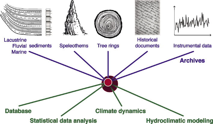Figure 1: Schematic illustration of the concept and goals of the PAGES’ Floods Working Group. Data on past floods will be collected from a variety of archive types, integrated into a database, statistically analyzed, and climatically modeled and interpreted.

Therefore, bringing together researchers from the growing community investigating past flood events worldwide is timely. A survey conducted in June 2015 by Wilhelm and Wirth, with support from PAGES, confirmed the need and interest in a Floods Working Group. The objective is to coordinate and synthesize results on the natural variability of floods under different climate conditions and in different regions of the world, plus offer an ideal platform to promote collaboration.

The leaders and the scientific committee defined four major goals for the first three-year period of the working group:

(i) Share best practice of methodologies used by the various research communities working with sediment records, tree rings, speleothems, instrumental data and more. The objective is to improve the quality of the flood records and to reduce uncertainties, for example in the detection of events and in the dating precision.

(ii) Intensify efforts for determining the magnitude of past floods reconstructed from natural archives via calibration with historical and instrumental data. Information on past flood magnitudes will highlight the importance of flood reconstructions for stakeholders and future flood-risk estimations.

(iii) Establish a database of published datasets on past floods. The goal of this open-access database will be to improve the visibility of existing paleo-flood data and to enable their intercomparison.

(iv) Test and identify optimal statistical tools for the analysis of flood frequency, occurrence of extremes, and the comparison of datasets.

A very important goal of the Floods Working Group during this first phase is also to promote interdisciplinary collaboration and discussion between flood scientists as well as specialists in the fields of hydrology, statistics, climate dynamics and modeling. This network will become particularly important to examine and model atmospheric processes and hydrological conditions leading to extreme floods.

We expect important links with the PAGES-endorsed Varves Working Group (pastglobalchanges.org/science/end-aff/varves-wg/intro), since varved lake sediments provide high-resolution and well-dated flood records. We also anticipate strong links with the PAGES 2k Network (pastglobalchanges.org/2k) as the density of flood data is high for the past 2000 years.

The Floods Working Group met for the first time at the “Cross Community workshop on past flood variability” in Grenoble, France, 27-30 June 2016. This workshop was held to gain an overview of the different kinds of flood archives and flood datasets that are available. Another key focus topic was the launch and management of the database, and to discuss visions and ideas of the participants. A report on this meeting will be published in the next issue of the PAGES Magazine.

affiliations

1Laboratoire d'Etudes des Transferts en Hydrologie et Environnement, University Grenoble Alpes, France

2Centre for Hydrogeology and Geothermics, University of Neuchâtel, Switzerland

3Dendrolab.ch, University of Bern, Switerland

contact

Bruno Wilhelm: bruno.wilhelmujf-grenoble.fr (bruno[dot]wilhelm[at]ujf-grenoble[dot]fr)

FWG: pastglobalchanges.org/floods