PAGES Magazine articles
Ken L. Ferrier1, W. van der Wal2, G.A. Ruetenik1 and P. Stocchi3
The movement of sediment across Earth’s surface affects sea level by deforming the solid Earth, modifying the gravity field, and displacing and absorbing water. Recent studies show that accounting for sediment redistribution is important for interpreting and predicting sea-level change.
Since the 19th century, it has been recognized that spatially variable sea-level changes result from changes in surface loading, which perturb Earth’s gravity field and the elevation of the crust (Jamieson 1865; Woodward 1888). Several decades ago, this connection was formalized in a gravitationally self-consistent theory of sea-level change (Farrell and Clark 1976), which, for the first time, accounted for both solid Earth deformation and the gravitational attraction of water toward itself, thus capturing the perturbations in both the sea floor and the sea surface that accompany ice melt. This theory has since been extended to account for several processes that were not included in Farrell and Clark’s classic study, including shoreline migration (Johnston 1993), Earth rotation (Milne and Mitrovica 1996), sediment redistribution (Dalca et al. 2013), and dynamic topography (Austermann and Mitrovica 2015).
To date, most applications of this theory have focused on sea-level responses to the growth and retreat of ice sheets, which produce the largest changes in surface loads over glacial-interglacial timescales. The retreat of the Laurentide ice sheet, for example, produced a rate of mass unloading ~102-103 times higher than that due to erosion in Earth’s most rapidly eroding mountain ranges.
Recent work has shown that sediment erosion and deposition, like ice growth and melt, produce significant changes in Earth’s crustal elevation, gravity field, and rotation axis, all of which induce changes in sea level. In this paper, we review the ways in which sediment redistribution affects sea level and demonstrate how this can improve our understanding of past sea-level change.
Processes and observations of sediment redistribution
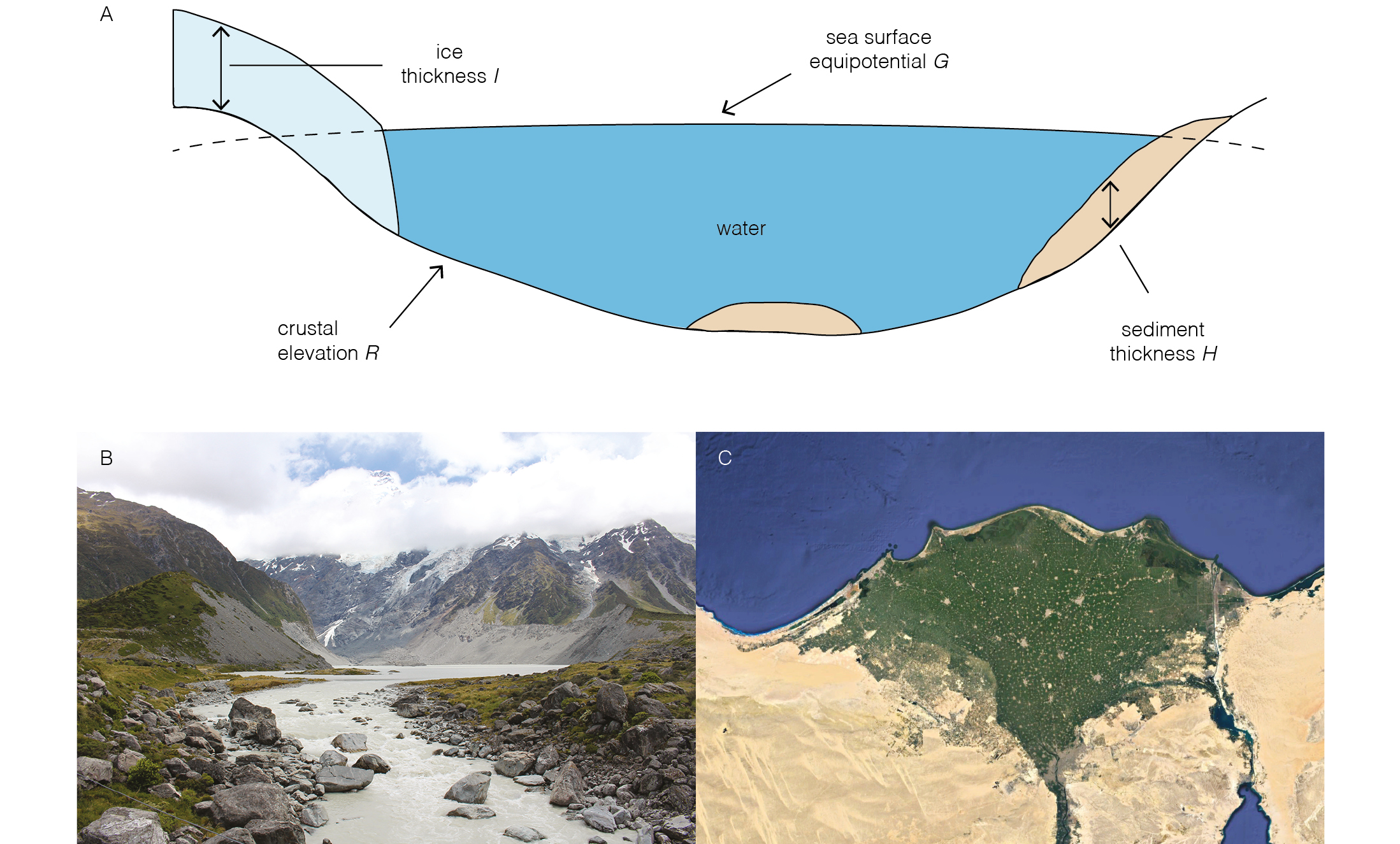
Sea-level responses to changes in surface loading are described by the sea-level equation (Eq. 1), which describes the change in sea level from one time to another, ΔSL (Fig. 1; Dalca et al. 2013).
ΔSL = ΔG – ΔH – ΔI – ΔR (1)
Here ΔH and ΔI are changes in the thicknesses of sediment and grounded ice, respectively, and are the drivers of sea-level change. ΔG and ΔR are changes in the elevations of the sea-surface gravitational equipotential and crust, respectively, and are responses to ΔH and ΔI that depend on Earth’s viscoelastic structure. Solid Earth responses to sediment redistribution over long timescales (>105 years) are often determined solely from the elastic flexure of the lithosphere, while responses over shorter timescales depend on the transient viscoelastic behavior of the mantle. Gravitational responses, by contrast, are essentially instantaneous, and continue evolving during sediment redistribution.
 |
|
Figure 1: (A) Components in the sea-level equation (Eq. 1). The largest influences of sediment on sea-level change are in places with rapid erosion, such as rapidly uplifting mountains, e.g. (B) the New Zealand Southern Alps, or rapid deposition, e.g. (C) the Nile Delta (Google Earth 2019). |
Quantifying ΔH requires establishing the rates and patterns of sediment erosion and deposition through time and space. At the largest scale, this includes erosion by fluvial, glacial, and hillslope processes, and deposition in subaerial floodplains, marine deltas, and fans. Integrated over the globe, these fluxes of sediment are large. Rivers currently carry ~18 ± 9 billion tons/year of sediment to the ocean (Willenbring et al. 2013), which is an order of magnitude smaller than ice-sheet mass change globally, but which can dominate changes in loading locally.
Because rates of erosion and deposition vary strongly in space, it is necessary to turn to empirical measurements to obtain realistic estimates of ΔH. Erosion rates are routinely inferred from fluvial sediment and solute fluxes, which provide rates averaged over annual to decadal timescales, and from cosmogenic nuclide concentrations in fluvial sediment, which yield rates averaged over ~103-105 years. Deposition rates are traditionally inferred from the age and thickness of sediment cores, which typically yield rates over ~102-105 years. Recently, new approaches have been developed to infer sediment deposition rates through remotely sensed perturbations in the gravity field (Mouyen et al. 2018). Although no single method can yield a continuous record of the history of erosion and deposition, the combination of methods provides useful constraints on the history of sediment redistribution over a range of timescales.
Effects of sediment redistribution and compaction on sea level and ocean water volume
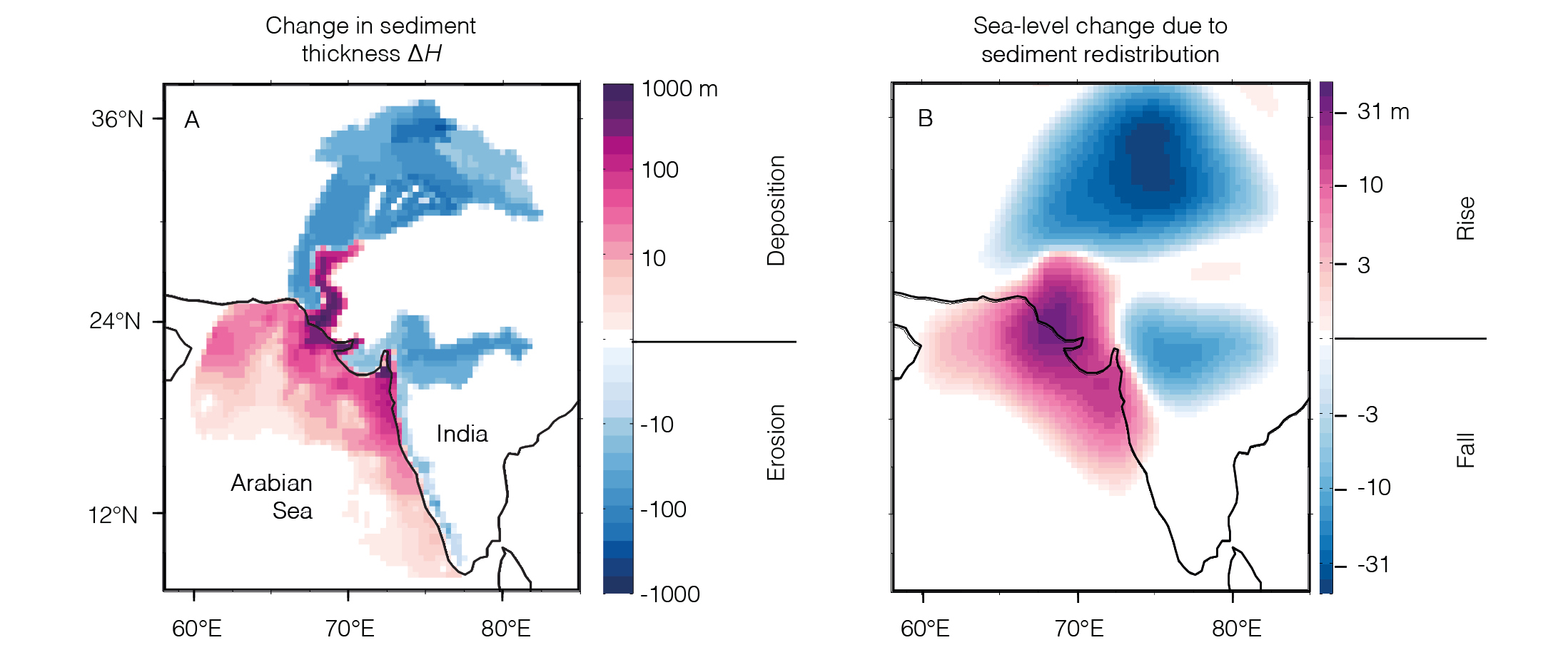
Figure 2 illustrates responses to sediment redistribution in a simulation of sea-level change driven by erosion in the Indus River basin and deposition in the Arabian Sea and the Indus plain (Ferrier et al. 2015). This produces a cumulative change in sediment thickness (ΔH) as large as hundreds of meters over the 122-kyr simulation (Fig. 2a) and a sediment flux from the Indus River of ~400 million tons/year, one of the largest fluvial sediment fluxes on Earth. This results in sea-level changes >30 m near the center of the Indus delta (Fig. 2b), implying that a hypothetical paleoshoreline that formed there during the Last Interglacial would now be submerged by tens of meters.
 |
|
Figure 2: (A) Cumulative changes in sediment thickness over a 122-kyr simulation dominated by rapid erosion in the western Himalaya and rapid deposition on the Indus delta and plain. (B) Modeled changes in sea-level (∆G – ∆R) due to sediment redistribution are as large as ~30 m, far exceeding published estimates of eustatic sea-level change over this period. This highlights the importance of accounting for the effects of sediment redistribution when using paleo sea-level markers to infer past sea-level change. Modified from Ferrier et al. (2015). |
The gravitationally self-consistent sea-level theory was recently extended (Ferrier et al. 2017) to account for two sedimentary effects that had long been recognized but not yet accounted for in the theory: the effects of sediment compaction on sediment thickness, and the effects of sedimentary water storage on global ocean water volume. Ferrier et al. (2018) applied this theory to a global sediment budget constrained by modern fluvial sediment fluxes, and showed that sedimentary water storage is capable of modifying the global volume of ocean water by the equivalent of ~2 ± 1 m in global mean sea level since the Last Interglacial, a significant fraction of the inferred 6-9 m drop in global mean sea level over this time (Kopp et al. 2009).
These sedimentary effects have important implications for interpreting past sea-level records. First, they imply that paleoshoreline elevations need to be corrected for the deforming effects of sediment, especially near locations of rapid deposition and erosion and over long time periods. Second, paleoshoreline-based inferences of past global ice volume need to properly account for changes in the volume of water stored in sediment.
Conclusions
Over the past five years, a number of studies have applied the gravitationally self-consistent sea-level theory to show that sediment redistribution can be a major driver of sea-level change. These studies have shown that sea-level responses are especially large in river systems with large sediment loads (Ferrier et al. 2015; Kuchar et al. 2018), and that sediment redistribution by other processes (e.g. subglacial erosion; van der Wal and IJpelaar 2017) can induce sea-level responses as well.
Several challenges remain. The history of sediment redistribution is poorly known in many locations due to limited measurements of paleo erosion rates, deposition rates, porosity, and density, especially for periods further in the past. In addition, lateral variations in mantle viscosity and lithospheric effective elastic thickness can strongly modulate sea-level changes, but exploring these effects is challenging due to uncertainties in Earth’s rheological structure and the computational expense of modeling sea-level responses on a laterally varying Earth. Such challenges motivate continued efforts to constrain the Earth’s sediment redistribution history and its three-dimensional structure, and to include erosion and deposition in coupled Earth system models that link climate forcings to sediment redistribution, glaciation, and sea-level change. Improved constraints on sediment redistribution, for example, may be useful in aiding interpretations of Gravity Recovery and Climate Experiment (GRACE) satellite data. Together, these studies highlight the rich behavior of sea-level responses to sediment redistribution, and reveal opportunities for improving our understanding of past and future sea-level change.
affiliations
1Department of Geoscience, University of Wisconsin-Madison, USA
2Faculty of Civil Engineering and Geosciences, Delft University of Technology, Netherlands
3Royal Netherlands Institute for Sea Research, Texel, Netherlands
contact
Ken Ferrier: kferrier wisc.edu
references
Austermann J, Mitrovica J (2015) Geophys J Int 203: 1909-1922
Dalca A et al. (2013) Geophys J Int 194: 45-60
Google Earth 7.3 (2019) 30.89°N, 31.09°E, viewing elevation 350 km. 3D map, satellite layer, viewed 1 March 2019, google.com/earth/index.html
Farrell W, Clark J (1976) Geophys J Int 46: 647-667
Ferrier K et al. (2015) Earth Planet Sci Lett 416: 12-20
Ferrier K et al. (2017) Geophys J Int 211: 663-672
Ferrier K et al. (2018) Geophys Res Lett 45: 2444-2454
Jamieson T (1865) Quart J Geol Soc London 21: 161-203
Johnston P (1993) Geophys J Int 114: 615-634
Kopp R et al. (2009) Nature 462: 863-867
Kuchar J et al. (2018) J Geophys Res Solid Earth: 123: 780-796
Milne GA, Mitrovica JX (1996) Geophys J Int 126: F13-F20
Mouyen M et al. (2018) Nat Commun 9: 3384
van der Wal W, IJpelaar T (2017) Solid Earth 8: 955-968
Bette L. Otto-Bliesner1, M. Lofverstrom2, P. Bakker3 and R. Feng4
The Last Interglacial is a recent warm interval with sea level higher than today. Climate modeling groups are simulating this time interval. Here, we illustrate feedbacks from vegetation changes and retreat of the Greenland ice sheet on regional responses to orbital forcing.
The Last Interglacial (LIG, 129 to 116 kyr BP; thousands of years before present, where present is defined as 1950 CE) is recognized as an important time interval for testing our knowledge of interactions between climate and ice sheets in warm climate states that led to deglaciation of the Greenland and potentially western Antarctic ice sheets. The LIG was already recognized as an important time period of relevance for the future in the First Assessment Report of the Intergovernmental Panel on Climate Change (IPCC; Folland et al. 1990). It gained more prominence since the Fourth and Fifth Assessment reports (IPCC AR4 and AR5) with new reconstructions highlighting that global mean sea level was ~6-9 m higher than present for several thousand years (Dutton et al. 2015). Questions remain regarding the contribution of the Greenland ice sheet to this highstand, as well as when and by how much temperatures peaked in the Northern Hemisphere high latitudes.
PMIP4-CMIP6 Last Interglacial simulations
Positive boreal summer insolation anomalies (with respect to present), associated with the orbital configuration of eccentricity, perihelion, and obliquity (Berger and Loutre 1991), occurred in the Northern Hemisphere from about 135 to 122 kyr BP, with maximum anomalies from 130 to 124 kyr BP. Anomalies were greater than 50 W/m2 for July at 65°N from 128 to 124 kyr BP. Correspondingly, negative austral summer insolation anomalies were present in the Southern Hemisphere. Antarctic ice-core records reveal that the greenhouse gas concentrations were relatively constant from 128 to 121 kyr BP; the atmospheric CO2 concentration was stable at pre-industrial values (about 280 ppmv) between 128 and 120 kyr BP (Schneider et al. 2013), while atmospheric CH4 concentrations peaked around 720 ppbv at ~128.5 kyr BP and then declined slowly (Loulergue et al. 2008).
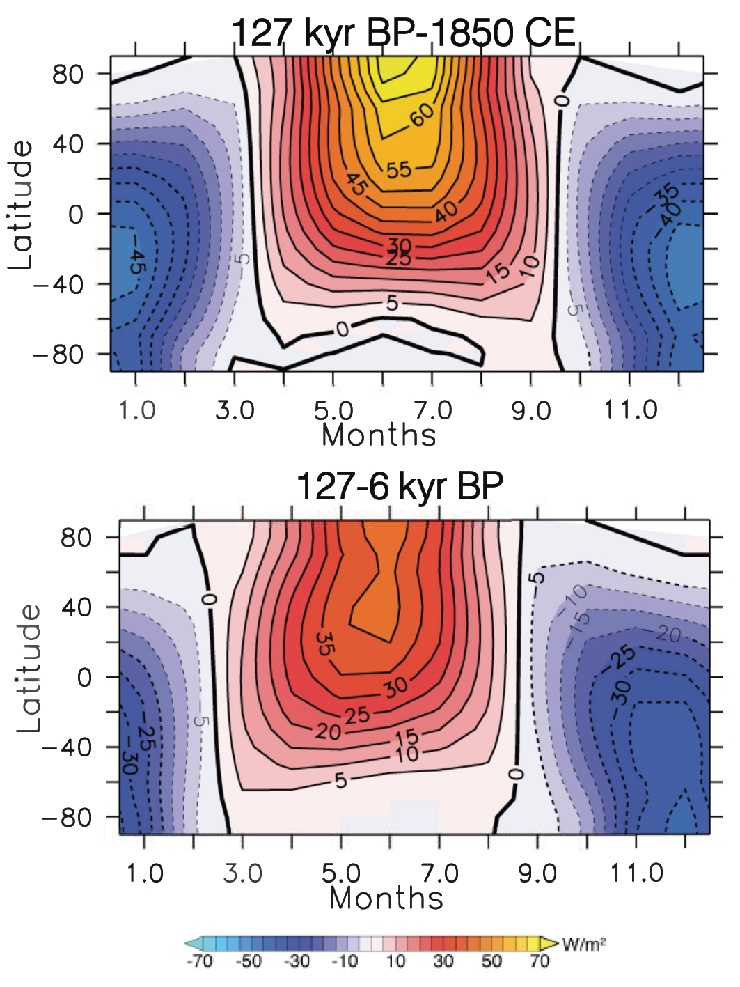
The suite of Paleoclimate Modelling Intercomparison Project (PMIP4) simulations in the Coupled Model Intercomparison Project (CMIP6) include a Tier 1 experiment for 127 kyr BP (lig127k; Otto-Bliesner et al. 2017). It is designed to address and compare the climate responses to orbital forcings stronger than the mid-Holocene experiment for 6 kyr BP (Fig. 1). The CMIP6 lig127k experiment will provide a basis to investigate the linkages between ice sheets and climate change in collaboration with the Ice Sheet Model Intercomparison Project for CMIP6 (ISMIP6; Nowicki et al. 2016).
The CMIP6 lig127k experiment is a time-slice (or equilibrium) experiment for 127 kyr BP. To provide a large ensemble of simulations from many international modeling groups, the boundary conditions are set to allow easy implementation in the same models used for the future scenarios of CMIP6. That is, the orbital parameters and greenhouse gas concentrations are set to represent 127 kyr BP, while the ice sheets (i.e. Greenland and Antarctica) and global land-ocean distribution are the same as in the pre-industrial control run (piControl). Although aerosols and vegetation may be interactive in some CMIP6 models, those without these capabilities are asked to use the same boundary conditions as in their piControl simulation.
Vegetation feedbacks
Vegetation during the LIG responded to the latitudinal and seasonal insolation changes associated with the orbital forcing. Pollen and macro-fossil evidence show that boreal forests extended farther north than today and, except in Alaska and central Canada, extended to the Arctic coast (CAPE 2006; LIGA 1991). Given the impact of increased forest cover on albedo and evapotranspiration, these vegetation changes, not included in the CMIP6 lig127k experiment unless models realistically simulate them interactively, could have had significant impacts on the surface energy budget in the Arctic, amplifying high-latitude warming (Swann et al. 2011).
 |
|
Figure 1: Latitude-month insolation anomalies for 127 kyr BP minus 1850 CE and 127 minus 6 kyr BP. |
To quantify the strength of this climate-vegetation feedback for explaining the inferred Arctic and Greenland warmth during the LIG, PMIP4-CMIP6 also includes a 127 kyr BP Tier 2 experiment where the vegetation cover at Northern Hemisphere high latitudes is changed from tundra to boreal forest. Simulations with the pre-release versions of the Community Earth System Model (CESM) v. 2.0 coupled to the Community Ice Sheet Model (CISM) v. 2.0 indicate that Arctic vegetation responses to the direct orbital warming are important for simulating high-latitude warming and sea-ice extent, and retreat of the Greenland ice sheet and its contribution to the LIG sea-level highstand.
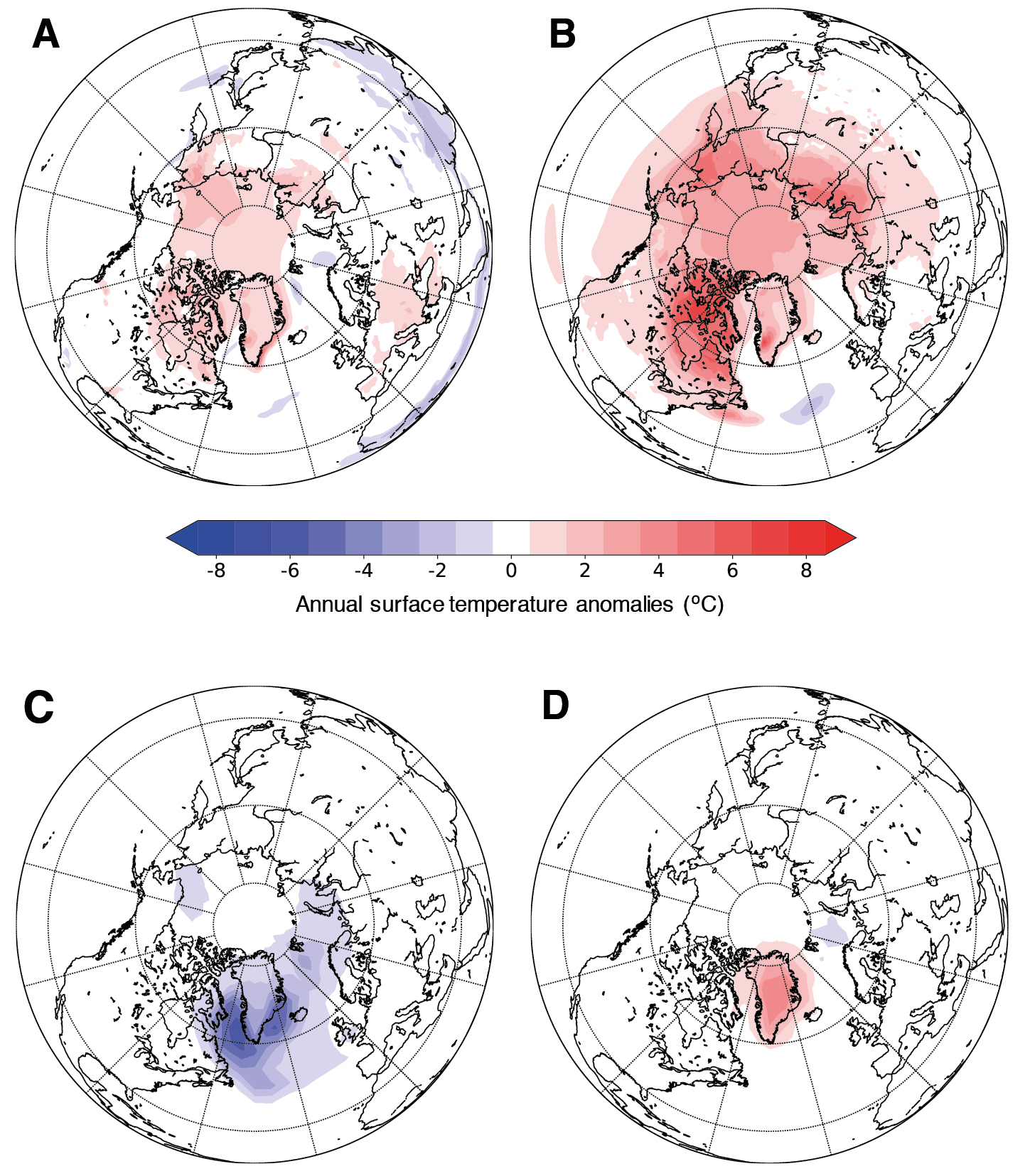
With orbital and GHG forcing only in a 127 kyr BP CESM-CISM simulation (Fig. 2a), the Arctic and Greenland are warmer than pre-industrial annually, but only modestly, by ~1-2°C over northern North America and northern Eurasia, and ~2°C in western Greenland. The memory of the cryosphere and positive feedbacks from changes in surface and cloud albedo amplify the warmer boreal summer temperatures and reduce sea-ice extent through the boreal winter months. The ice sheet over Greenland retreats minimally in western Greenland, retaining most of the modern ice-sheet area. The overall Greenland surface-mass balance remains positive with Greenland contributing only about 0.5 m of equivalent global sea-level change over 3000 years. The global, annual surface temperature change is ~0°C, similar to the results of LIG simulations assessed in the IPCC AR5 (Masson-Delmotte et al. 2013).
With the prescribed high-latitude vegetation change of the 127 kyr BP Tier 2 experiment, the simulated annual warming increases in the Arctic, particularly over northern Siberia and northeast Canada, where the feedback between vegetation and surface warming is responsible for an additional warming of ~4-8°C (Fig. 2b). Annual surface temperature change compared to the pre-industrial control run in the northwest of Greenland is greater than 4°C and in the southwest greater than 7°C. After 3000 years of 127 kyr BP forcing and feedbacks, the Greenland ice sheet has retreated significantly along its west periphery, with a total ice-sheet area of ~85% of modern and contributing ~2 m sea level equivalent to the LIG highstand.
 |
|
Figure 2: Annual surface temperature anomalies (°C) as simulated by climate models for the Last Interglacial. (A) LIG (orbital and GHG forcing) minus PI (preindustrial control); (B) LIGveg (LIG plus high-latitude tundra replaced by boreal forest) minus LIG; (C) LIGmwf (LIG plus Greenland meltwater to North Atlantic) minus LIG; and (D) LIGgris (LIG plus albedo and topography changes for retreat of Greenland ice sheet) minus LIG. (A) and (B) are from 127 kyr time-slice simulations with CESM-CISM, (C) and (D) are from 130 kyr BP time-slice simulations with LOVECLIM. |
Effects of the retreating Greenland ice sheet
Other slow feedbacks are also important for explaining regional Arctic and Greenland changes. As the Greenland ice sheet retreats under warmer summer temperatures, meltwater is discharged into the North Atlantic Ocean. This freshwater has the potential to slow down the Atlantic Meridional Overturning Circulation (AMOC) and cool the North Atlantic and surrounding continental regions, depending on the rate and amount of meltwater discharged. Thus, meltwater resulting from the retreat of the Greenland ice sheet can provide a negative feedback to the orbital warming. Simulations for 130 kyr BP with the LOVECLIM model (Bakker et al. 2012) indicate a reduction of the deep convection and cooling of ~4-6°C in the Labrador Sea when a constant runoff flux of 0.05 Sv, equivalent to 2.3 m of Greenland melt, is added for 500 years to ocean grid cells surrounding Greenland (Fig. 2c). Warmer July surface temperatures as compared to pre-industrial still persist over the Nordic Seas and Europe. Lowering the Greenland ice sheet, on the other hand, results in a local warming over Greenland of up to 4°C (Fig. 2d).
Future outlook
Uncertainties in the boundary conditions for the LIG suggest that the PMIP4-CMIP6 lig127k simulation, designed to maximize the multi-model ensemble size, may not capture important feedbacks for explaining the observed Arctic warmth and for assessing the contribution of the Greenland ice sheet to the LIG sea-level highstand. Future Earth system models will need to include next-generation dynamic global vegetation models with considerations of climate, soil, and vegetation competition; a Greenland ice-sheet model with predictive ice-ocean interactions; and eventually solid Earth models, in order to simulate both fast and slow feedbacks of the entire Earth system on the transient evolution of the Greenland ice sheet during the Last Interglacial. Equally important will be new LIG reconstructions detailing the range and composition of vegetation at high latitudes, volume and flow pattern of the Greenland ice sheet, volume and extent of sea ice, and state of the ocean circulation.
affiliations
1Climate and Global Dynamics Laboratory, National Center for Atmospheric Research, Boulder, USA
2Department of Geosciences, University of Arizona, Tucson, USA
3Department of Earth Sciences, Vrije Universiteit Amsterdam, The Netherlands
4Center for Integrative Geosciences, University of Connecticut, Storrs, USA
contact
Bette L. Otto-Bliesner: ottobliucar.edu
references
Bakker P et al. (2012) Clim Past 8: 995-1009
Berger A, Loutre M-F (1991) Quat Sci Rev 10: 297-317
CAPE-Last Interglacial Project Members (2006) Quat Sci Rev 25: 1383-1400
Dutton A et al. (2015) Science 349: aaa4019
LIGA members (1991) Quat Int 10-12: 9-28
Loulergue L et al. (2008) Nature 453: 383-386
Nowicki SM et al. (2016) Geosci Model Dev 9: 421-4545
Otto-Bliesner BL et al. (2017) Geosci Model Dev 10: 3979-4003
Bas de Boer1, F. Colleoni2, N.R. Golledge3 and R.M. DeConto4
Numerical ice-sheet models are a key tool to estimate the contribution of ice sheets to past sea-level change. Here, we highlight a few developments and applications of ice-sheet models that allow ice-sheet contributions to past sea-level changes to be estimated.
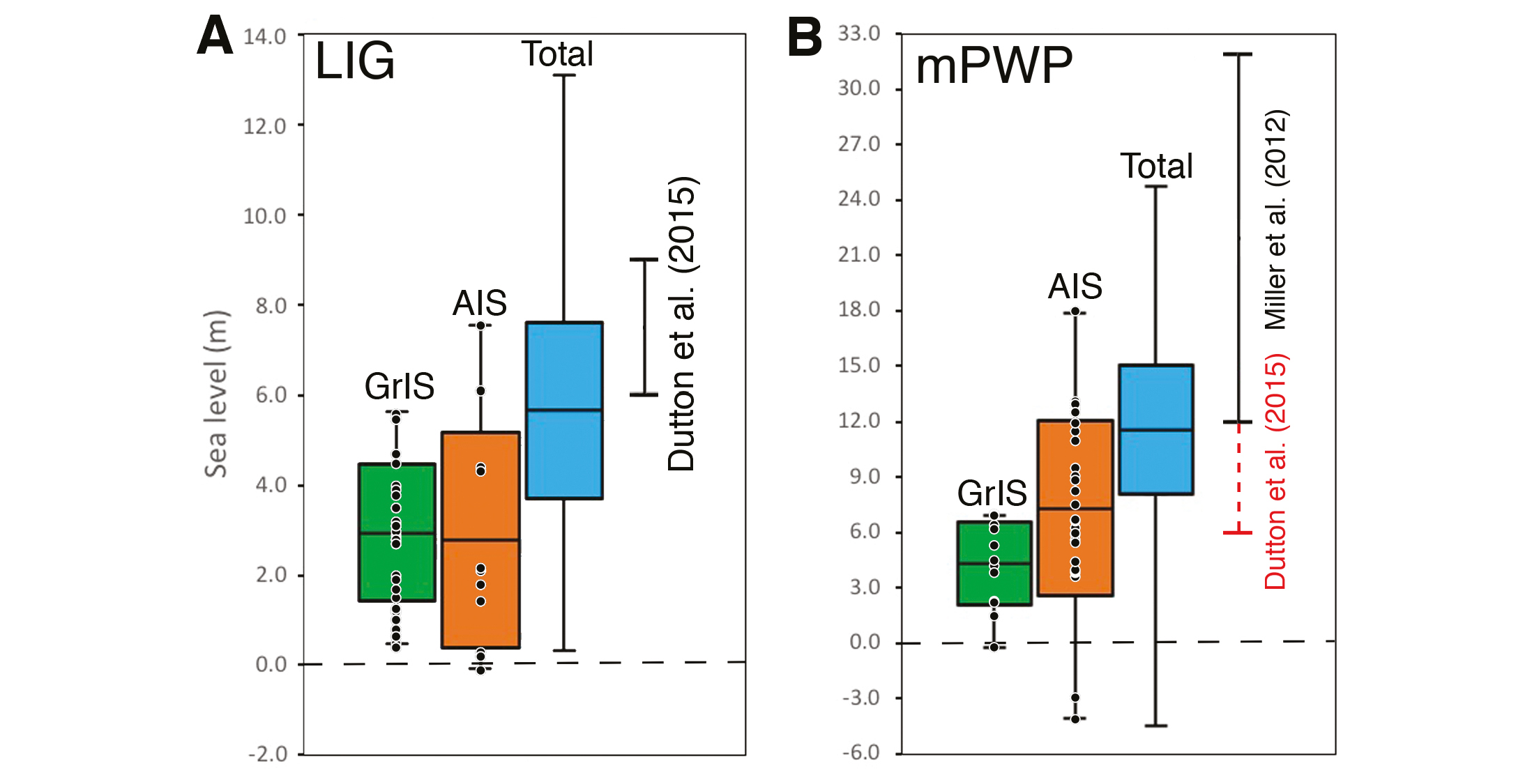
Past warm intervals such as the mid-Piacenzian Warm Period (mPWP: 3.264-3.025 million years ago) or the Last Interglacial (LIG: 129-116 thousand years (kyr) ago) have been widely studied to constrain past sea-level changes (e.g. Sutter et al. 2016; de Boer et al. 2017). Also, those intervals are studied for process understanding of the Earth system as an analogue for future warming (e.g. DeConto and Pollard 2016). Geological evidence indicates that global mean sea level during the mPWP and LIG were likely to be up to 20 m or more (Miller et al. 2012) and 6-9 m (Dutton et al. 2015) relative to the present, respectively. This reflects the cumulative (a)synchronous contribution of the Greenland and Antarctic ice sheet (GrIS and AIS). Numerical ice-sheet models are the only means to determine their individual contribution to past sea-level changes.
Ice sheets in the climate system
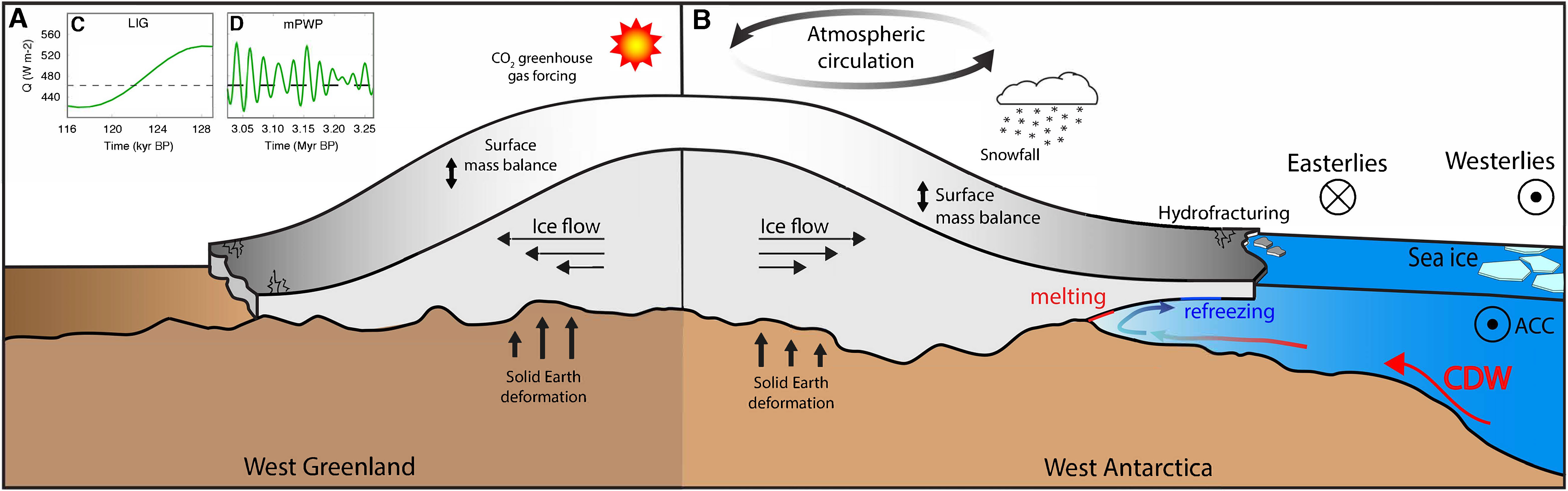
Over the past decades, critical aspects of ice-sheet models related to the interactions with the ocean, the atmosphere, basal hydrology, and the solid Earth, have been substantially improved. The mass budget of the ice sheets is largely affected by processes that act at the interface between these different systems (Fig. 1). Of the present mass budget of the GrIS, surface melting accounts for 60% of the mass loss (van den Broeke et al. 2016). During the mPWP (besides increased greenhouse gases) and the LIG, higher summer insolation (Fig. 1c,d) can increase mass loss significantly and induce ice-sheet retreat (e.g. Robinson and Goelzer 2014; de Boer et al. 2017).
 |
|
Figure 1: Schematic representation of an ice sheet that (A) terminates on land. Heavy crevassing at the edges, insolation, snowfall, and temperature control the mass balance. (B) Schematic of an ice sheet that terminates at the ocean. Melting at the grounding line is induced due to intrusion of CDW in the cavities underneath the ice shelves. Hydrofracturing and sub-shelf melting dominate the mass balance of ice shelves that buttress the ice sheet. Inset shows insolation at June 65°N (Laskar et al. 2004) during (C) the LIG (129-116 kyr ago) and (D) the mPWP (3.264-3.025 Myr ago). The horizontal dashed line shows present insolation at 462.29 W m-2. |
The ocean plays a key role in AIS changes (e.g. Sutter et al. 2016; Golledge et al. 2017), largely due to the fact that large sectors of the bed lie well below sea level. Punctuated intrusion of relatively warm and saline ocean water – Circumpolar Deep Water (CDW) – underneath the ice shelves (Fig. 1b) enhances ice-shelf basal melting and thinning, leading to a significant contribution to the mass loss of ice shelves. Under warm climatic conditions, climate models show that intrusion of CDW is fostered by a southward shift and strengthening of the westerly winds, which leads to a more vigorous Antarctic Circumpolar Current (ACC), and increases sub ice-shelf melting (see also Fig. 4 in Colleoni et al. 2018).
Development of paleo ice-sheet models
The basic principles that enable the use of 3D ice-sheet models for long-term paleoclimate applications involve the adoption of approximate flow equations (i.e. the shallow ice and shallow shelf approximations). This allows for relatively fast calculations (e.g. 100 kyr in a few hours), on coarse grids of 20-40 km, of continental-scale ice sheets. Complex atmospheric or oceanic interactions would require coupling (a)synchronously with a climate model, but are still computationally too expensive. Therefore, in stand-alone ice-sheet models, atmospheric and oceanic variations are crudely parameterized, and long-term transient evolution in surface air temperatures and precipitation usually follows reconstructions of ice-core or benthic oxygen isotope records (e.g. Huybrechts 2002; de Boer et al. 2017).
To determine the surface mass balance, long-term paleo ice-sheet simulations rely on simple parametrizations of snow accumulation and surface melting. Melt can be computed using the Positive Degree Day method (PDD), which uses only temperature (e.g. Huybrechts 2002), or alternatively accounting for insolation forcing on surface melt through the Insolation Temperature Melt (ITM) model (e.g. Robinson and Goelzer 2014). PDD and ITM are computationally inexpensive parameterizations and capture the glacial-interglacial behavior of continental-scaled ice sheets, but differences can be large relative to full energy balance models (e.g. Plach et al. 2018).
Similarly, for the ice-shelf-ocean interface, long-term ice-sheet simulations rely on local heat-balance parameterizations using a vertically uniform oceanic temperature, or a spatially varying field based on present-day observations (e.g. DeConto and Pollard 2016). More complex schemes are being developed, such as plume-melt models (Lazeroms et al. 2018), which account for the interaction with the local geometry and the spatially varying oceanic temperatures, or ocean box models, directly coupled to ice-sheet models, which simulate the overturning circulation in ice-shelf cavities (Reese et al. 2018). Accordingly, model developments are critical to improve calculation of GrIS and AIS contribution to past and future sea-level variations.
Modeling past sea level from the GrIS and AIS
Over recent decades, numerous studies have estimated the contribution to past sea level from the GrIS and AIS (Fig. 2). Different approaches have been used, using either a single surface-air temperature anomaly or steady state climate forcing, transient or equilibrium simulations, or fully coupled to a (lower resolution) climate model (see for example overviews in Dutton et al. 2015; Dolan et al. 2018; Plach et al. 2018). The broad range of simulated individual contributions from the GrIS and AIS clearly illustrate the uncertainties related to the use of different ice-sheet and climate models to estimate past sea-level changes (as also shown in Dolan et al. 2018).
 |
|
Figure 2: Overview of published sea-level contributions (in meters) from the GrIS (green) and AIS (orange). (A) The LIG compared with the range from Dutton et al. (2015) and (B) the mPWP compared with the range from Dutton et al. (2015) in red, and Miller et al. (2012) in black. Simulations are shown by the black dots in (A) and (B); sources are listed in the online supplementary material. From each source we used either one value or the mean value of an ensemble, including the range. Boxes indicate the total mean, with one standard deviation. The maximum and minimum modeled ice sheet within the total ensemble are indicated by the whiskers (in black). Totals (blue) are calculated by summing the mean, minimum and maximum and averaging the standard deviations from the GrIS and AIS. References listed below. |
The total mean sea-level change estimated from ice-sheet models is on the low end compared to the geological evidence for both the LIG and the mPWP (blue boxes in Fig. 2a,b). A higher contribution from the LIG AIS could stem from interactions with the ocean (e.g. Sutter et al. 2016), although two-way interaction with the climate cannot be ignored. The driving processes leading to increased ice-cliff calving are not yet fully understood but could account for a significant retreat of the LIG and mPWP AIS (DeConto and Pollard 2016), whereas gaps in knowledge of the subglacial topography leads to greater uncertainties for AIS contribution to mPWP sea level (Gasson et al. 2015). Surface melt of the GrIS can be significantly enhanced relative to the present due to increased summer insolation (Fig. 1c,d) during the mPWP and LIG (Robinson and Goelzer 2014; de Boer et al. 2017).
Outlook
Precisely quantifying the impact of processes, such as calving and ice-cliff failure, on the GrIS or AIS and the impact of the interaction between ocean warming and sub-glacial topography on ice-sheet retreat remains challenging (DeConto and Pollard 2016). Nonetheless, more precisely located and time-varying geological data will allow for a much more detailed study of coupled paleo ice-sheet climate simulations. This might reduce model-data discrepancies and lead to a consensus of past sea-level contributions from the GrIS and AIS in the coming years, thus providing stronger constraints to future sea-level projections.
affiliations
1Faculty of Science, Earth and Climate, Vrije Universiteit Amsterdam, The Netherlands
2National Institute of Oceanography and Experimental Geophysics, Trieste, Italy
3Antarctic Research Centre, Victoria University of Wellington, New Zealand
4Department of Geoscience, University of Massachusetts Amherst, USA
contact
Bas de Boer: bas.de.boervu.nl
references
Colleoni F et al. (2018) Nat Commun 9:2289
Dolan AM et al. (2018) Nat Commun 9:2799
de Boer B et al. (2017) Geophys Res Lett 44: 10,486-10,494
DeConto RM, Pollard D (2016) Nature 531: 591-597
Dutton A et al. (2015) Science 349: aaa4019
Huybrechts P (2002) Quat Sci Rev 21: 203-231
Gasson et al. (2015) Geophys Res Lett 42: 5372-5377
Golledge NR et al. (2017) Geophys Res Lett 44: 2343-2351
Laskar J et al. (2004) Astron Astroph 428: 261-285
Lazeroms WMJ et al. (2018) Cryosphere 12: 49-70
Miller KG et al. (2012) Geology 40: 407-410
Plach A et al. (2018) Clim Past 14: 1463-1485
Reese R et al. (2018) Cryosphere 12: 1969-1985
Robinson A, Goelzer H (2014) Cryosphere 8: 1419-1428
Sutter J et al. (2016) Geophys Res Lett 43: 2675-2682
van den Broeke MR et al. (2016) Cryosphere 10: 1933-1946
Figure 2
LIG - GrIS
Letréguilly A et al. (1991) Palaeogeogr Palaeocl Palaeoecol 90: 385-394
Ritz C et al. (1996) Clim Dynam 13: 11-23
Cuffey KM, Marshall SJ (2000) Nature 404: 591-594
Huybrechts P (2002) Quat Sci Rev 21: 203-231
Tarasov L, Peltier WR (2003) J Geophys Res 108: 2143
Lhomme N et al. (2005) Quat Sci Rev 24: 173-194
Greve R (2005) Ann Glaciol 42: 424-432
Otto-Bliesner BL et al. (2006) Science 311: 1751-1753
Fyke J et al. (2011) Geosci Model Dev 4: 117-136
Robinson A et al. (2011) Clim Past 7: 381-396
Born A, Nisancioglu KH (2012) Cryosphere 6: 1239-1250
Stone EJ et al. (2013) Clim Past 9: 621-639
Quiquet A et al. (2013) Clim Past 9: 353-366
Helsen MM et al. (2013) Clim Past 9: 1773-1788
de Boer B et al. (2014) Nat Commun 5: 3999
Calov R et al. (2015) Cryosphere 9: 179-196
Goelzer H et al. (2016) Clim Past 12: 2195-2213
Tabone I et al. (2018) Clim Past 14: 455-472
Bradley SL et al. (2018) Clim Past 14: 619-635
LIG - AIS
Huybrechts P (2002) Quat Sci Rev 21: 203-231
Pollard D, DeConto RM (2009) Nature 458: 329-332
Pollard D, DeConto RM (2012) Geosci Model Dev 5: 1273-1295
de Boer B et al. (2014) Nat Commun 5: 3999
Goelzer H et al. (2016) Clim Past 12: 2195-2213
Sutter J et al. (2016) Geophys Res Lett 43: 2675-2682
DeConto RM, Pollard D (2016) Nature 531: 591-597
mPWP - GrIS
Lunt DJ et al. (2008) Nature 454: 1102-1105
Hill DJ et al. (2010) Stratigraphy 7: 111-122
Koenig SJ et al. (2015) Clim Past 11: 369-381
Contoux C. et al. (2015) Earth Planet Sci Lett 424: 295-305
Dolan AM et al. (2015) Clim Past 11: 403-424
de Boer B et al. (2015) Cryosphere 9: 881-903
de Boer B et al. (2017) Geophys Res Lett 44: 10,486-10,494
mPWP - AIS
Pollard D, DeConto RM (2009) Nature 458: 329-332
Pollard D, DeConto RM (2012) Geosci Model Dev 5: 1273-1295
de Boer B et al. (2014) Nat Commun 5: 3999
de Boer B et al. (2015) Cryosphere 9: 881-903
Austermann J et al. (2015) Geology 43: 927-930
Gasson E et al. (2015) Geophys Res Lett 42: 5372-5377
Yan Q et al. (2016) J Geophys Res 121: 1559-1574
DeConto RM, Pollard D (2016) Nature 531: 591-597
Golledge NR et al. (2017) Clim Past 13: 959-975
Jacqueline Austermann1 and Alessandro M. Forte2
Mantle flow pushes Earth's surface up or drags it down, causing kilometer-scale topographic anomalies. As this so-called “dynamic topography” evolves, it can influence local sea level and the sensitivity of ice sheets to climate change.
Local sea-level reconstructions have been the foundation for understanding past ice-sheet behavior, especially records spanning the last deglaciation and past interglacial periods. Linking the evolution of local sea level to global mean sea level, which is also related to ice-volume changes, requires a correction for any uplift or subsidence of the field site that has occurred since the sea-level record was formed. Such vertical movements can occur due to tectonic crustal deformation, glacial isostatic adjustment (GIA; e.g. Milne et al. this issue), erosion, or sediment loading (e.g. Ferrier et al. this issue).
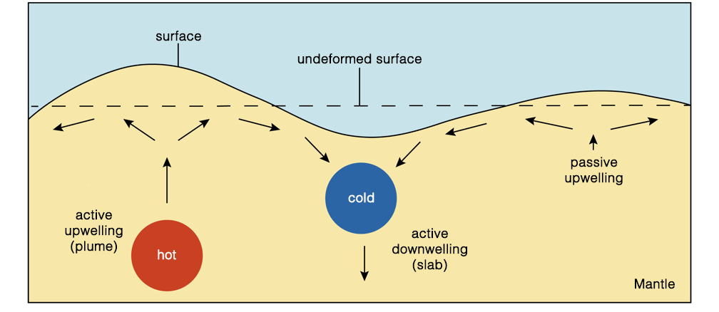
Another process that shapes Earth's surface is dynamic topography, which is the topography generated by vertical forces arising from buoyancy-induced flow within the Earth's mantle (Fig. 1). While this process was first recognized decades ago, the full extent to which dynamic topography affects sea-level records over the Plio-Pleistocene and interacts with the Earth climate system as a whole (e.g. ice sheets and oceans) has only recently been explored.
 |
|
Figure 1: Illustration of how flow in the mantle can generate dynamic surface topography (modified from R. Moucha, personal communication). |
Definition of mantle dynamic topography
Today's surface topography is shaped by crustal isostasy, in which, for example, crustal roots support mountain belts, and dynamic topography, which is driven by stresses in the sub-crustal mantle that are caused by (shallow) isostatic and (deeper) flow-driven contributions (Forte et al. 1993). Both of these components evolve with time as lateral density variations in the sub-crustal mantle convect and cool the rocky mantle. This leads to spatio-temporal changes in dynamic topography that contribute to the evolution of Earth's surface.
While convection extends from the lithosphere to the core-mantle boundary, sensitivity studies reveal that density heterogeneity in the shallow mantle (e.g. the lithosphere and asthenosphere) contributes most to the overall topographic signal (Forte et al. 2015). The definition of dynamic topography used here includes the topographic signature of the lithosphere (e.g. cooling and subsidence of the oceanic lithosphere), as it constitutes the upper thermal-boundary layer of Earth's convective interior. However, it is important to note that a lithospheric signal is sometimes removed from models or observations in order to investigate sub-lithospheric or deep-mantle drivers of surface topography.
Present-day dynamic topography
Estimates of present-day dynamic topography can be obtained by removing the crustal isostatic effect from the observed topography, which requires knowledge of the crustal thickness and density, as well as overlying sediment, water, and ice loads. Global estimates of dynamic topography reveal large-scale undulations with magnitudes that exceed 2 km (Forte et al. 2015). Within the oceans, a detailed assessment has shown that the sub-lithospheric contribution to dynamic topography has a magnitude that ranges from approx. -1.5 km (Australia-Antarctic discordance) to 2 km (around Iceland) and can have steep lateral gradients (e.g. 1 km of dynamic topography change over a lateral distance of 1000 km along the West African Margin; Hoggard et al. 2016).
These observations of dynamic topography can be used to improve numerical models of mantle convection and understand the dynamics of the Earth's interior. Models of present-day mantle convection require an input density field of the Earth's interior (estimated from seismic tomography), a rheological constitutive equation that describes the relationship between deformation and stress, and boundary conditions, which govern the tangential stresses at the surface and core-mantle boundary. Assuming conservation of mass and momentum, one can determine the instantaneous velocity and dynamic stress fields (Forte et al. 2015). The resulting dynamic topography is calculated by balancing radial stresses at the Earth's surface (Fig. 1). Current mantle convection models provide satisfactory fits to the present-day observations of dynamic topography and gravity anomalies (Simmons et al. 2010); however, debate over the largest and small-scale features still exists (Hoggard et al. 2016).
Changes of dynamic topography
To understand the role of dynamic topography in sea-level reconstructions, we are interested in the temporal evolution of dynamic topography, rather than its absolute (present-day) value. Importantly, present-day amplitudes do not provide information on the change of dynamic topography through time. For example, locations that are dynamically supported today are equally likely to be uplifting or subsiding.
Changes in dynamic topography can be deduced from a variety of geological and geomorphological data. For example, a careful analysis of stratigraphy from onshore and offshore Australia indicates changes in dynamic topography (subsidence) of up to 75 m/Myr on the Northwest Shelf (Czarnota et al. 2013). Paleo shorelines from the US east coast, Australia, and South Africa indicate rates of uplift of up to 20 m/Myr (Rovere et al. 2014). Model-derived estimates of the rate of change in dynamic topography can vary from a few meters per million years (Flament et al. 2013) up to over 100 m per million years (Rowley et al. 2013; Austermann et al. 2017) depending on the model input parameters, particularly the viscosity structure, magnitude of density perturbations, and whether density variations in the asthenosphere and lithosphere are considered.
The contribution of dynamic topography to past sea-level and ice-sheet changes
Initial indications that dynamic topography can cause local sea-level changes stems from observations and modeling work on continental flooding histories over the Phanerozoic (Bond 1979; Gurnis 1993). It is now recognized that local paleo sea-level reconstructions, whether from continental flooding, backstripping at passive margins, or stratigraphy in sedimentary basins, are not equal to global mean sea-level change, due to regionally varying changes in dynamic topography (Moucha et al. 2008). This limitation also applies to the more recent past of the Plio-Pleistocene.
 |
|
Figure 2: Model results of dynamic topography (DT) change since the last interglacial period from (A) the mean of 12 different models (Austermann et al. 2017) and (B) one preferred model scenario for the US east coast (Dutton and Forte 2016) based on mantle convection reconstructions by Glišović and Forte (2016). |
Mapping of Pliocene shorelines shows significant variations in their elevations relative to one another and along the shoreline feature (Rovere et al. 2014). The most prominent example is the Orangeburg Scarp along the US east coast, which exhibits a change in elevation of up to 40 m after correcting for glacial isostatic adjustment. Rowley et al. (2013) have shown that this relative deformation can be explained by changes in dynamic topography. However, uncertainties in input parameters for numerical models of dynamic topography, as well as an incomplete understanding of the contribution of competing deformation processes, such as sediment loading, still hinder a quantification of global mean sea level and, hence, ice-sheet stability during this time period. This work prompted a re-examination of sea-level records from earlier interglacials. Model predictions indicate that dynamic topography can contribute up to several meters of deformation to local sea-level records dating to the last interglacial period (Fig. 2). This modeling is corroborated by a significant correlation between the predicted deformation and the observed elevations of sea-level indicators from the last interglacial (Austermann et al. 2017). Estimates of excess global mean sea level during this time period are 6-9 m (Dutton et al. 2015), which does not account for dynamic topography. If key sites have been affected by changes in dynamic topography, this 6-9 m estimate could be incorrect by a few meters. Improving estimates of global mean sea level and ice-sheet stability during past interglacials therefore hinges on a better understanding of dynamic topography.
Mantle flow underneath ice sheets can also directly affect ice-sheet evolution. For example, dynamic topography changes along the grounding line of the Antarctic Wilkes Basin potentially made this sector more susceptible to retreat in the Pliocene epoch (Austermann et al. 2015).
Mantle flow directly affects sea-level records, ice-sheet behavior, and ocean dynamics, which has led to intriguing new links between the solid Earth and the climate system. This nascent connection provides promising avenues to potentially answer some open questions in paleoclimate research, as well as the opportunity to expand observational constraints on the structure and dynamics of Earth's deep interior.
acknowledgements
We would like to thank A. Dutton and M. Hoggard for many helpful discussions. AMF acknowledges support provided by the University of Florida and thanks P. Glisovic (GEOTOP, UQAM) for his contributions and for support from the Natural Sciences and Engineering Research Council of Canada and Calcul Québec.
affiliations
1Lamont-Doherty Earth Observatory, Columbia University, New York City, USA
2Department of Geological Sciences, University of Florida, Gainesville, USA
contact
Jacqueline Austermann: ja3170columbia.edu
references
Austermann J et al. (2015) Geology 43 : 927-930
Austermann J et al. (2017) Science Advances 3: e1700457
Bond GC (1979) Tectonophysics 61: 285-305
Czarnota K et al. (2013) Geochem Geophy Geosy 14: 634-658
Dutton A et al. (2015) Science 349: aaa4019
Dutton A, Forte A (2016) AGU Fall Meeting, PP51B-2309
Flament N et al. (2013) Lithosphere 5: 189-210
Forte AM et al. (1993) Geophys Res Lett 20: 225-228
Glišović P, Forte AM (2016) J Geophys Res: Solid Earth 121, 4067-4084
Gurnis M (1993) Nature 364: 589-593
Hoggard M et al. (2016) Nat Geosci 9: 456-463
Moucha R et al. (2008) Earth Planet Sci Lett 271: 101-108
Rovere A et al. (2014) Earth Planet Sci Lett 387: 27-33
Glenn A. Milne1, D. Al-Attar2, P.L. Whitehouse3, O. Crawford2 and R. Love4
We overview two PALSEA-relevant applications of glacial isostatic adjustment modeling and highlight recent advances. These include the consideration of models with lateral Earth structure and the development of methods to determine optimal parameters and model uncertainty.
The primary aim of the PALSEA (PALeo constraints on SEA level rise) working group is to promote and improve the use of constraints from observations and modeling of past sea-level changes and ice-sheet extent to better inform projections of future sea-level change. Glacial isostatic adjustment (GIA) – the deformational, gravitational and rotational response of the Earth to past ice-sheet evolution – plays an important role in reaching this objective in several respects (see Editorial, this issue). Here we review recent advances in two key PALSEA-relevant GIA model applications - estimating global ice volume during past warm periods and the contribution of GIA to future sea-level change - and consider recent developments towards improving uncertainty estimation in GIA model output which is central to these applications.
Estimating global ice volume during past warm periods
A core aim of PALSEA is to estimate the peak in global mean sea level (GMSL), from which global ice volume can be inferred, during past warm periods when GMSL was greater than at present. There are three periods in relatively recent Earth history for which observations indicate that GMSL was above the present value: the Mid-Pliocene warm period (~3 Myr BP), Marine Isotope Stage 11 (~420-370 kyr BP), and Marine Isotope Stage 5e (~129-116 kyr BP; the Last Interglacial). Estimating GMSL from a sparse distribution of local relative sea level (RSL) indicators is non-trivial due to under-sampling and the fact that local sea level can depart significantly from the global mean value. GIA is one of a number of processes (e.g. dynamic topography and sediment loading; see contributions on these topics in this issue) that should be considered when estimating GMSL from RSL records. A small number of studies have demonstrated that the GIA “overprint” can significantly bias estimates of GMSL for each of the three warm periods mentioned above (e.g. Raymo et al. 2011; Raymo and Mitrovica 2012; Kopp et al. 2009; Dutton and Lambeck 2012; Dendy et al. 2017). Specifically, they show that the GIA contribution to RSL can range from order 1-10 m depending on the data location and the choice of model inputs (parameters).
Regarding model inputs, the ice-loading history and Earth viscosity structure are the most important. There is considerable uncertainty in both of these, so it is necessary to perform model-sensitivity analyses to map out which parametric uncertainty dominates at the specific data locations. The analysis of Dendy et al. (2017) is the most thorough in this respect. In addition to uncertainty in model parameters, limitations in the model itself, due to, for example, missing processes or simplifications in the geometry, can lead to considerable error or bias in the output (formally known as model structural error). A recent advancement in this area is the development of coupled models that account for feedbacks between GIA-related processes and ice dynamics (see Whitehouse 2018). One limitation in all of the GIA studies noted above is the use of spherically symmetric Earth models in which parameters vary only with depth. GIA models that include a 3D Earth structure have been applied in some studies that consider post-Last Glacial Maximum sea levels or geodetic observations (Whitehouse 2018) and the impact has been shown to be non-negligible. However, the computational expense of these models currently prohibits their use for earlier times such as those mentioned above due to the longer time integrations required.
 |
|
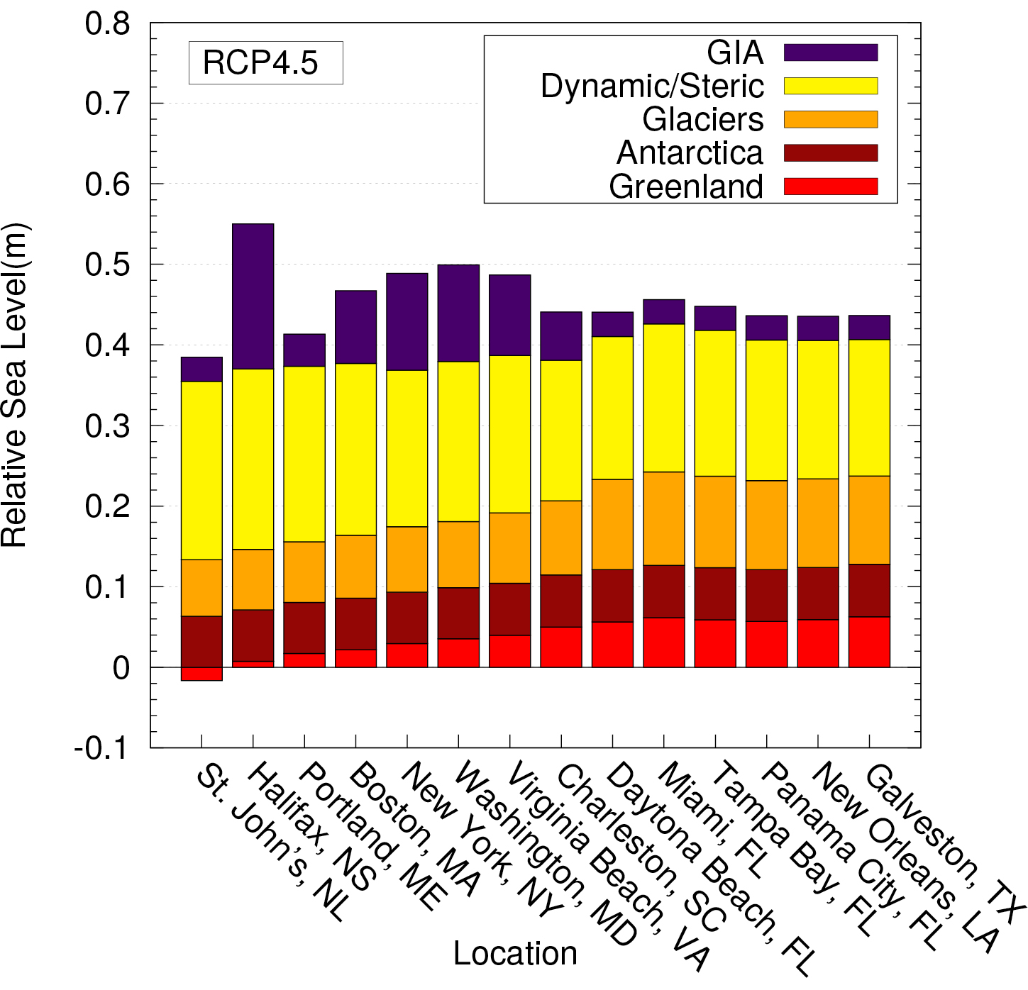
Figure 1: Regional sea-level projections for 2085–2100 relative to 2006–2015 for the intermediate representative concentration pathway (RCP) 4.5. The future contribution from melting of land ice is determined from the respective sea-level fingerprints of the Antarctic and Greenland ice sheets as well as the global distribution of glaciers and ice caps. The contribution from ocean circulation (dynamic) and steric changes is also shown. Figure adapted from Love et al. (2016). |
The contribution of GIA to future sea-level change
The construction of comprehensive regional RSL projections, which requires the compilation and summation of contributions from different processes, has only been attempted relatively recently (e.g. Slangen et al. 2014). In regions that were recently deglaciated, GIA will be a significant contributor to future RSL change. The GIA component has been either explicitly included using process model output (Slangen et al. 2014) or estimated from tide-gauge records as part of a linear trend that could also include other secular processes (for example, tectonics; Kopp et al. 2014). In the former case, one issue has been the lack of accurate uncertainty estimates on GIA model output.
Recent studies (Love et al. 2016; Yousefi et al. 2018) have sought to address this issue by using a large suite of model runs sampling a broad range of Earth and ice-model parameters as well as a state-of-the-art regional RSL database to estimate model uncertainty. The PALSEA-led effort to produce regional RSL databases using standard protocols (Khan et al. this issue) has greatly enhanced the quality and availability of these databases, facilitating improved GIA model development. The studies of Love et al. (2016) and Yousefi et al. (2018) demonstrate the relative importance of GIA for future sea-level change along the Atlantic and Pacific coasts of North America (e.g. Fig. 1) and, perhaps more importantly, that uncertainty in defining the GIA contribution is large and that spherically symmetric Earth models are not able to accurately reproduce observations of recent RSL change in these regions.
 |
|
Figure 2: The sensitivity of modeled sea level in Tahiti (as marked by the cross) 9000 years ago to perturbing the background mantle viscosity structure at a depth of 1756 km. The background viscosity structure is scaled from a tomographic model of seismic shear wave-speed variations using a simple empirical relation. Results for other depths and times, when combined, define sensitivity kernels that can be used to invert RSL data from Tahiti for an optimal 3D viscosity model with uncertainty estimates (Crawford et al. 2018). |
Towards improved GIA models
Two key aspects of GIA model development relevant to the applications outlined above include the use of Earth models that can accommodate lateral Earth structure as well as methods to estimate model parameters and the uncertainty associated with each. Past studies have used large ensemble forward modeling and statistical methods to estimate uncertainty in the ice (e.g. Tarasov et al. 2012) and spherically symmetric Earth models (e.g. Caron et al. 2017). Given the interdependence of these model inputs, future analyses should aim to jointly infer ice- and Earth-model parameters and their uncertainty. Estimating parametric uncertainty is more challenging with 3D Earth models given the much larger parameter space and the uncertainty in constraining lateral viscosity structure (Whitehouse 2018).
A step towards overcoming the latter issue is the determination of sensitivity kernels for GIA observables. These kernels quantify the linearized dependence of observations on underlying parameters, and can be used in both inversions and uncertainty quantification (Fig. 2). Early studies estimated such kernels using finite-difference approximations (e.g. Zhong et al. 2003), but here the computational cost scales with the number of model parameters, and so rapidly becomes infeasible. A better approach is through the use of the adjoint method, which produces exact kernels at the cost of just two forward simulations (Al-Attar & Tromp 2014). Using this approach, the inversions for ice history and 3D Earth structure from GIA observables is a realistic goal, with promising synthetic tests having been performed recently (Crawford et al. 2018; Fig. 2).
affiliations
1Department of Earth and Environmental Sciences, University of Ottawa, Canada
2Department of Earth Sciences, University of Cambridge, UK
3Department of Geography, Durham University, UK
4Department of Physics and Physical Oceanography, Memorial University of Newfoundland, St John’s, Canada
contact
Glenn A. Milne: gamilneuottawa.ca
references
Al-Attar D, Tromp J (2014) Geophys J Int 196: 34–77
Caron L et al. (2017) Geophys J Int 209: 1126-1147
Crawford O et al. (2018) Geophys J Int 214: 1324–1363
Dendy J et al. (2017) Quat Sci Rev 171: 234-244
Dutton A, Lambeck K (2012) Science 337 : 216-219
Kopp RE et al. (2009) Nature 462: 863-867
Kopp RE et al. (2014) Earth’s Future 2: 287–306
Love R et al. (2016) Earth’s Future 4: 440-464
Raymo ME et al. (2011) Nat Geosci 4: 328-332
Raymo ME, Mitrovica JX (2012) Nature 483: 453-456
Slangen ABA et al. (2014) Clim Change 124: 317-332
Tarasov L et al. (2012) Earth Planet Sci Lett 315-316: 30-40
Whitehouse PL (2018) Earth Surf Dyn 6:401-429
Louise C. Sime1, A.E. Carlson2 and M. Holloway1,3,4
The sensitivity of the Antarctic ice sheet to ocean warming is a major source of uncertainty in projecting future sea levels. Antarctic ice from the Last Interglacial sampled in ice cores provides key information to better quantify this sensitivity.
Quantifying the sensitivity of the Antarctic ice sheet (AIS) to increasing ocean temperatures is central to improving projections of global sea-level rise. Capron et al. (2014) compiled strong evidence of a Southern Ocean sea-surface temperature anomaly of up to +3.9 ± 2.8°C 125,000 years ago (125 kyr BP) compared to the present, and sea-level indicators for the Last Interglacial (LIG; around 129 to 116 kyr BP) suggest that this was the last time that global mean sea level (GMSL) was substantially higher than present (Dutton et al. 2015). This strongly suggests that pinning down the response of the AIS during the LIG should give insight into the last time the AIS was substantially smaller than today.
Ice-sheet modeling, alongside other lines of evidence, suggest the potential for massive loss of West Antarctic ice that is grounded below sea level (e.g. DeConto and Pollard 2016). Isotopic analysis of marine sediments and the NEEM Greenland ice core indicate that Greenland likely provided a relatively small ~2 m contribution to maximum LIG sea levels (NEEM Project Members 2013; Colville et al. 2011), so the reconstructed LIG GMSL peak of +6 to 9 m implies that the AIS experienced very significant melt during the LIG (Dutton et al. 2015). However, hunting for more direct evidence of AIS changes during the LIG has thus far proved to be surprisingly difficult, and the ultimate goal of deriving rates of AIS volume change has yet to be achieved.
Terrestrial observations of the extent of the AIS during the LIG are lacking due to subsequent growth of the AIS to its last glacial maximum volume. However, some evidence exists in the marine realm to constrain the LIG AIS. A tephra layer in the ANDRILL sediment core from the Ross Sea shows that at some time in the last 240 kyr, the Ross ice shelf was absent, potentially during the LIG (McKay et al. 2012). According to some ice-modeling studies, if the Ross ice shelf was to completely melt, the West Antarctic ice sheet (WAIS) would also deglaciate (e.g. DeConto and Pollard 2016). A recent study from a marine core off East Antarctica used Neodynium isotopes to show that the portion of the AIS overlying the Wilkes subglacial basin significantly retreated to a smaller-than-present extent during the LIG (Wilson et al. 2018). While similar studies near other sectors of the AIS could provide fruitful information on the LIG extent of the AIS, none of these approaches have, on their own, permitted the definitive establishment of AIS changes during the LIG.
The attractions of ice-core data
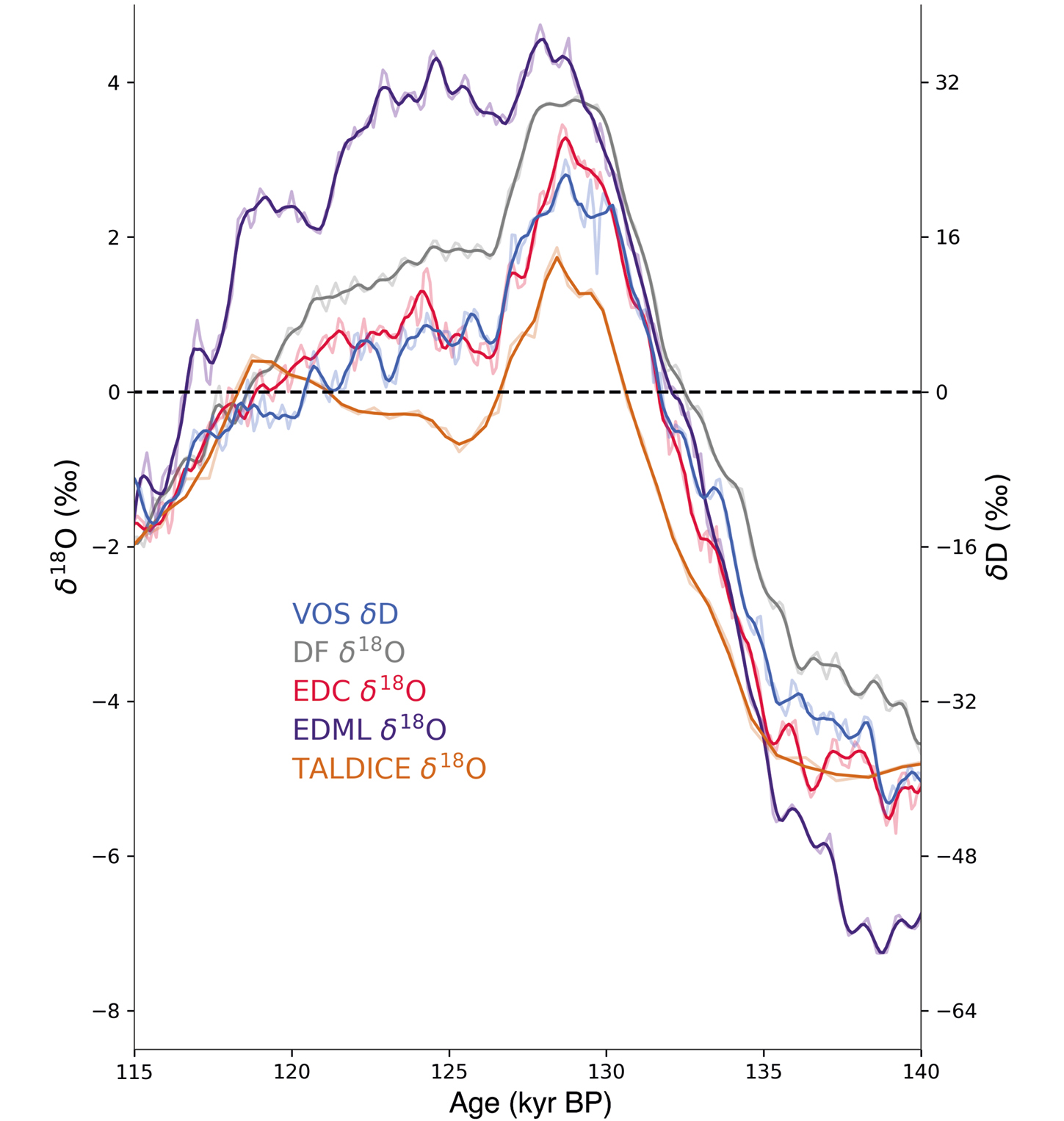
Antarctic ice cores are an attractive proposition for reconstructing AIS changes: several ice cores from East Antarctica covering the LIG period have been placed on an improved chronology using new gas and ice stratigraphic links (Bazin et al. 2013). The age uncertainty on this improved chronology is approximately 1500 years during the LIG, which is excellent compared to most other LIG data. Air content measurements from such ice cores have been used to attempt to infer changes in East Antarctic surface elevation over the past 200 kyr (e.g. Martinerie et al. 1994). However, Bradley et al. (2012) demonstrated that existing East Antarctic ice-core sites would experience negligible elevation change in response to a past WAIS collapse, and unknowns in firn modeling make the conversion from air content to atmospheric pressure, needed to infer elevation changes, highly uncertain. However, water isotope (δ18O) data has been measured with a precision generally better than 0.1‰ on these same ice cores. These well-dated and precise measurements (Fig. 1) hold the tantalizing prospect of establishing accurate rates of AIS change during the LIG.
 |
|
Figure 1: Last interglacial (~129-116 kyr BP) δD and δ18O anomalies (relative to the most recent 3 kyr BP) from the Vostok (VOS), Dome Fuji (DF), EPICA Dome Concordia (EDC), EPICA Dronning Maud Land (EDML), and Talos Dome (TALDICE) ice-core records. Raw ice-core data (light lines) are shown as well as a smoothed record (dark lines). The locations (filled circles) of these ice cores are shown in Figure 2. |
Steig et al. (2015) and Holloway et al. (2016) tackled the question of whether changes in the AIS, particularly ice loss from West Antarctica, would exert a significant control over the δ18O signal recorded in Antarctic ice cores. Using δ18O-enabled climate modeling, both demonstrated that significant West Antarctic mass loss or gain would cause major changes that should be observable in ice cores from both West and East Antarctica. Key patterns in ice-core δ18O can be generated by melt from the AIS via resulting influences on atmospheric circulation, sea surface temperatures, and sea-ice extent around Antarctica (Holloway et al. 2017).
All of these aspects exert a strong and readily identifiable influence on δ18O at the Antarctic ice-core sites (Holloway et al. 2016, 2018).
Constraints from ice-core data thus far
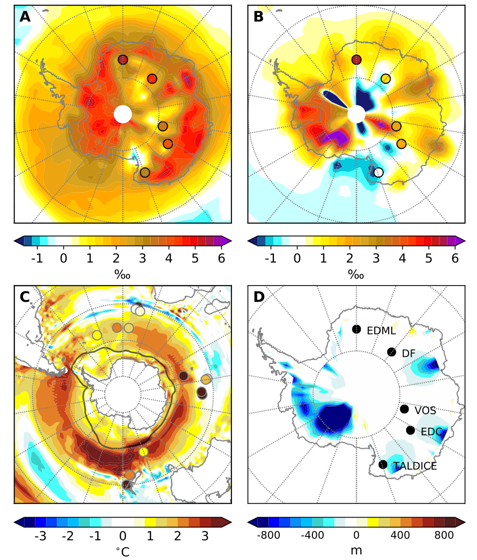
Holloway et al. (2016) investigated whether the distinctive peak in δ18O observed in ice cores at ~128 kyr BP (Fig. 1) was due to the loss of West Antarctic ice, but concluded that it was extremely likely that the WAIS was largely still intact at 128 kyr BP. A recent extension of this work (Holloway et al. 2018) using a fully coupled, isotope-enabled climate model demonstrates that the reconstructed penultimate deglacial meltwater event (around 0.2 Sv of meltwater input to the North Atlantic region over around 4 kyr) appears to explain the peak at 128 kyr BP in δ18O, via the well-known bipolar seesaw mechanism; these results indicate that meltwater input over ~3600 years can generate the whole ice-core δ18O signal at 128 kyr BP (Fig. 2a). The succession of events is thus: (i) Meltwater from Northern Hemisphere ice sheets caused warming of the Southern Ocean; (ii) This in turn melted Antarctic sea ice over a period of around 3-5 kyr BP; and (iii) The loss of sea ice subsequently imprinted itself on the ice cores as a peak in δ18O (Holloway et al. 2017). This work also indicates that the climate models used here appear to be capable of accurately capturing key timings and processes during past warm periods.
 |
|
Figure 2: (A) Anomalies in Antarctic δ18O from a 128 kyr BP HadCM3 climate model experiment relative to the corresponding pre-industrial experiment. (B) As in (A) but for a 125 kyr BP experiment including no meltwater forcing and Antarctic ice-sheet topography equivalent to the minimum ice-sheet extent (DeConto and Pollard 2016). (C) Simulated summer (JFM) sea surface temperature anomalies (reconstructed anomalies from Capron et al. (2014) are shown as filled circles) and winter sea-ice extent scaled corresponding to (A). (D) Antarctic elevation anomalies corresponding to (B) and locations of measured ice-core δ18O anomalies shown in (A), (B), and Figure 1. See Holloway et al. (2018) for more details. |
Of course, the work described above does not address the main aim, which is to uncover AIS change throughout the entire LIG. In particular, determining how the AIS may have responded after the 128 kyr BP ice-core δ18O peak (itself a response to the reconstructed Southern Ocean warming and sea-ice retreat; e.g. Fig 2c) is yet to be a focus of ice-core modeling research (e.g. Holloway et al. 2016). The research performed to date does, however, provide key results to build upon:
• It establishes confidence in both climate models and in our understanding of LIG atmosphere and ocean dynamics. It also means that we now know with some confidence that the LIG δ18O peak (shown in Fig. 1) was caused primarily by Antarctic sea-ice retreat in response to relatively high Southern Ocean temperatures, themselves generated by meltwater from the penultimate deglaciation.
• It indicates that the AIS was likely resilient to higher-than-present sea surface temperatures and reduced Antarctic sea ice during the early LIG, since the AIS was largely intact at 128 kyr BP. Parts of the AIS could, however, have melted shortly after 128 kyr BP (e.g. Fig. 2b) in direct response to the warming, but this has yet to be established.
Next steps
Focused study on the period following the ice-core δ18O peak (~125 kyr BP; Fig. 1) may provide important information on the magnitude and timescales of AIS change in response to a period of reduced sea ice and Southern Ocean warming. An example is illustrated in Figure 2b; ice-core δ18O data at 125 kyr BP may be better explained using a reduced AIS configuration relative to present day, suggesting substantial continental ice loss in the 3 kyr period following the reconstructed LIG Antarctic sea-ice minimum.
Based on these recent advances, we suggest that the next steps should include: (i) checking, using δ18O-enabled models, how ice cores may respond to other types and magnitudes of AIS changes (e.g. Fig. 2b), (ii) assessing whether our current ice-core data are sufficient to establish AIS changes; and (iii) obtaining new LIG ice-core data as necessary to constrain the models. Once these steps have been taken, we may find ourselves in a position to be able to pin down the most likely timing and contribution of the AIS to GMSL during this past warm interval.
affiliations
1Ice Dynamics and Paleoclimate, British Antarctic Survey, Cambridge, UK
2College of Earth, Ocean, and Atmospheric Sciences, Oregon State University, Corvallis, USA
3Data Science Division, National Physical Laboratory, Teddington, UK
4School of Geographical Sciences, University of Bristol, UK
contact
Louise C. Sime: lsimbas.ac.uk
references
Bazin L et al. (2013) Clim Past 9: 1715-1731
Bradley S et al. (2012) Glob Planet Change 88-89: 64-75
Capron E et al. (2014) Quat Sci Rev 103: 116-133
Colville EJ et al. (2011) Science 333: 620-623
DeConto RM, Pollard D (2016) Nature 531: 591-597
Dutton A et al. (2015) Science 349: aaa4019
Holloway MD et al. (2016) Nature Commun 7: 12293
Holloway MD et al. (2017) Geophys Res Lett 44: 11,129-11,139
Holloway MD et al. (2018) Geophys Res Lett 45: 11,921-11,929
Martinerie P et al. (1994) J Geophys Res 99: 10565-10576
McKay R et al. (2012) Quat Sci Rev 34: 93-112
NEEM Project Members (2013) Nature 493: 489-494
Anders E. Carlson1 and Nicolaj K. Larsen2,3
The Greenland ice sheet has the capacity to raise sea level by ~7.4 m. Current terrestrial and marine data suggest that the ice sheet has usually been smaller than present during interglacial periods, showing a high sensitivity to current regional climate warming.
The Greenland ice sheet is the last surviving ice sheet of what was the order-of-magnitude larger extent of North Hemisphere ice sheets at the last glacial maximum about 21,000 years ago. As such, its responses to ongoing and future global warming represents a major concern regarding its impact on global sea level. In the last decade, the application of 10Be exposure dating along with “threshold” lakes dated by 14C now constrain the timing of when the Greenland ice sheet retreated to a smaller-than-present extent in the Holocene. Likewise, radiogenic isotopic tracers of silt-size particles combined with ice-rafted debris and subglacial bedrock cosmogenic isotopic concentration can provide evidence of how small the Greenland ice sheet may have been in prior interglacial periods. These data can provide important constraints on the sensitivity of the Greenland ice sheet to paleoclimates similar to, or warmer than, present.
The Holocene
The last deglaciation leading into the Holocene is characterized by abrupt climate changes recorded in Greenland ice cores. However, evidence for any response of Greenland ice-sheet margins on land is restricted mainly to the southernmost, westernmost and easternmost edges of Greenland; other terrestrial retreat of the Greenland ice sheet occurred during the Holocene (e.g. Young et al. 2013; Carlson et al. 2014; Larsen et al. 2015, 2018; Winsor et al. 2015; Young and Briner 2015; Sinclair et al. 2016; Reusche et al. 2018). This means that at an extended state on the continental shelf, the Greenland ice sheet appears to have been relatively stable and capable of surviving 10,000 years of deglacial warming before retreating to its current and then smaller-than-present extent.
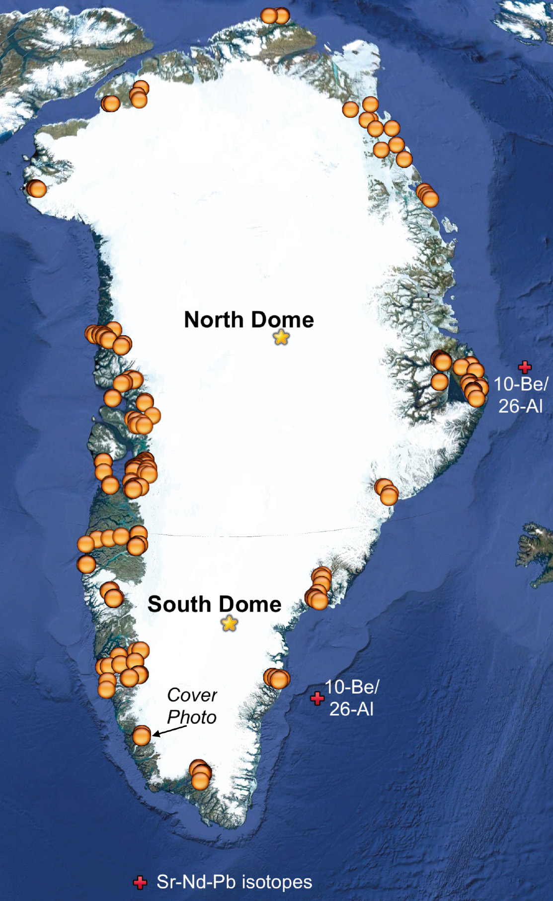
The application of 10Be exposure dating in a number of fjord transects (Fig. 1) has demonstrated that the deglaciation from the coast to the present ice margin occurred in most places within ~500-1000 yr during the early Holocene (e.g. Winsor et al. 2015; Young and Briner 2015; Sinclair et al. 2016; Larsen et al. 2018). These yield retreat rates of 50-100 m yr-1, which are similar to, or higher than, retreat rates observed at even the most sensitive glaciers today (Winsor et al. 2015). In west and southwest Greenland, the ice-sheet retreat halted during the early Holocene in response to the ~9.3 kyr BP and 8.2 kyr BP cold events (e.g. Young et al. 2013; Winsor et al. 2015). Elsewhere in Greenland, evidence of early Holocene stillstands is lacking – not necessarily because they did not occur, but because late-Holocene advance may have overridden moraines from these stillstands (Carlson et al. 2014; Larsen et al. 2015, 2018; Sinclair et al. 2016; Reusche et al. 2018).
 |
|
Figure 1: Location of 10Be ages (yellow circles), basal ice and bedrock samples (stars), and marine sediment cores (red crosses) constraining Greenland ice-sheet paleo history. Location of issue cover photo from Nigerdlikasik Bræ denoted by arrow. |
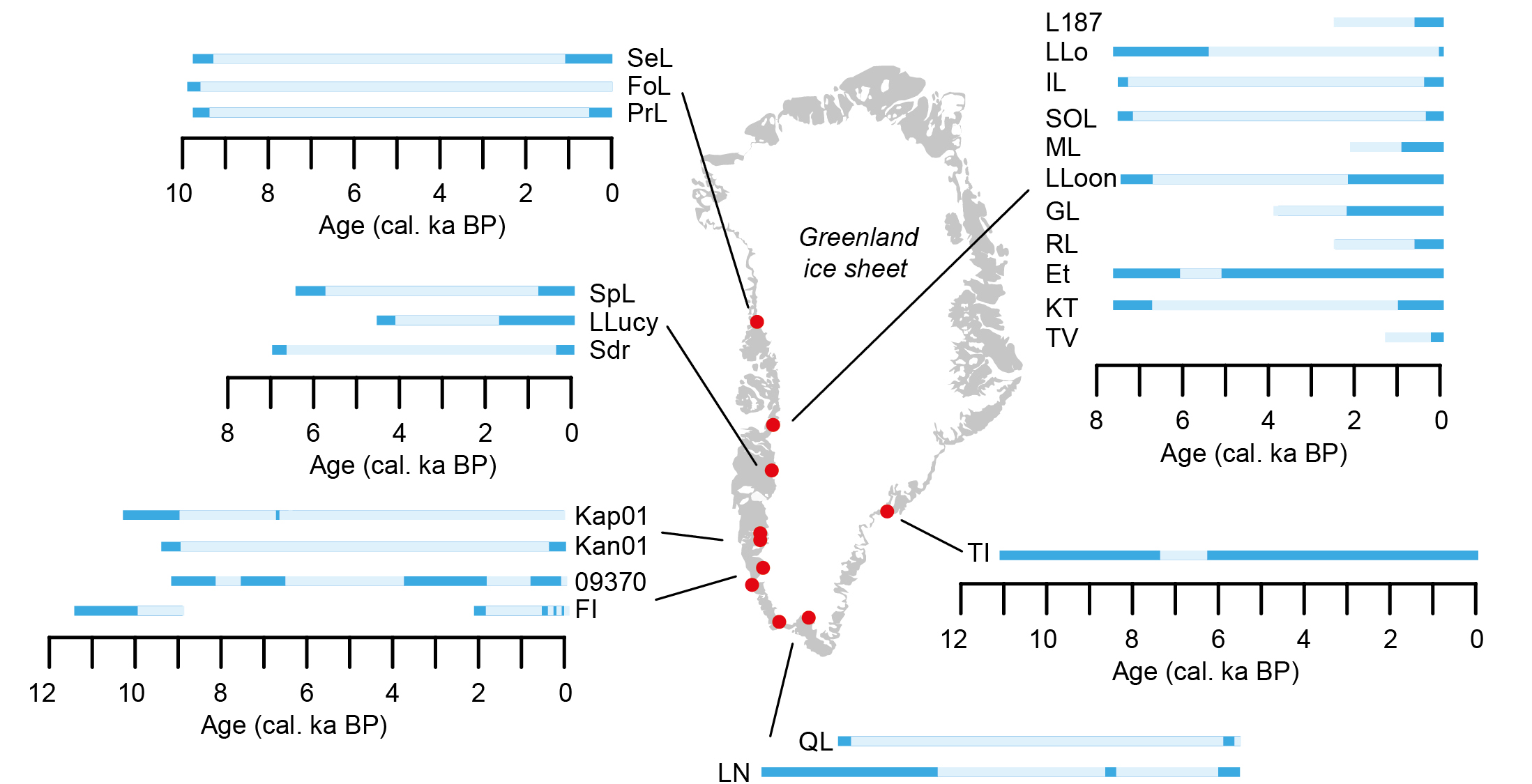
Cosmogenic ages on boulders next to modern ice margins (Fig. 1) and threshold lakes (Fig. 2), and radiocarbon dating on organic remains in historical moraines have been used to constrain periods with smaller-than-present ice extent (e.g. Carlson et al. 2014; Larsen et al. 2015; Young and Briner 2015). These records show that ice had retreated inland of its present extent during the Holocene thermal maximum ~8-5 kyr BP. This minimum ice extent was followed by a late-Holocene advance that culminated during the early 1900s with the formation of pronounced Little Ice Age moraines in most parts of Greenland (Kjeldsen et al. 2015). However, 10Be dating of moraines outside Little Ice Age moraines has shown that the ice extent was larger prior to the Little Ice Age in southernmost (Winsor et al. 2014) and northwestern Greenland (Reusche et al. 2018). These records indicate that for much of the last 10,000 years the Greenland ice sheet was at a more retracted extent than it was in the industrial era.
Prior interglacial periods
The last interglacial period, ~128-116 kyr BP, was an interval generally denoted as warmer than the peak Holocene due to greater precession forcing. Far-field sea-level indicators suggest that global mean sea level was 6-9 m above present, indicating that the global cryosphere was smaller than present. Marine sediment provenance records can constrain ice-sheet location on a given Greenland terrain (Colville et al. 2011). The dating of basal ice by the accumulation of radionuclide gases emitted from the underlying ground provides another means of reconstructing the Greenland ice sheet extent (Yau et al. 2016). The marine provenance records show that the southern Greenland ice dome survived through the last interglacial period (Fig. 1; Colville et al. 2011). The age of basal ice for the southern and northern Greenland domes is much older than the last interglacial (Fig. 1; Yau et al. 2016), in agreement with the marine records. These records suggest that the Greenland ice sheet only contributed less than 2.5 m (~35% of the modern ice-sheet volume; Colville et al. 2011) to the last interglacial sea-level highstand.
 |
|
Figure 2: Examples of Holocene constraints on when the Greenland ice sheet was smaller than present based on proglacial threshold lakes (Young and Briner 2015; Larsen et al. 2015 and reference therein). Dark bars indicate that the ice margin is close to the lake and similar to the modern extent; light bars indicate ice-margin retreat out of the lake drainage basin and a smaller-than-present ice extent. |
Prior to the last interglacial period, marine sediment provenance evidence indicates that the southern Greenland ice sheet nearly completely deglaciated during marine isotope stage 11 ~400 kyr BP (Reyes et al. 2014). This agrees well with the ~400 kyr BP age of basal ice and sediment from the south Greenland ice dome (Fig. 1; Yau et al. 2016). With a basal ice age of ~1000 kyr BP for the north Greenland ice dome (Fig. 1; Yau et al. 2016), these records suggest up to 6 m of sea-level rise coming from the Greenland ice sheet during marine isotope stage 11, accounting for the low end of global mean sea-level estimates for this interglacial period (Reyes et al. 2014).
On a longer timescale, marine and sub-ice cosmogenic records appear to be contradictory. For east Greenland, ice-rafted debris has been continuously deposited over the last three million years. The accumulation of 10Be and 26Al in this ice-rafted debris suggests the general persistence of the north Greenland ice dome in east Greenland over this time period with only short-lived periods of ice retreat and bedrock exposure (Fig. 1; Bierman et al. 2016). This would agree with the basal ice age of north Greenland ice dome of ~1000 kyr BP, suggesting a stable north Greenland ice dome over the latter part of the Quaternary (Yau et al. 2016). Conversely, the accumulation of 10Be and 26Al in the bedrock underlying the north Greenland ice dome could indicate multiple intervals of exposure during the Quaternary (Fig. 1; Schaefer et al. 2016), which would imply a more dynamic ice dome than can be inferred from the marine 10Be and 26Al records (Bierman et al. 2016) and basal ice ages (Yau et al. 2016). However, the eastern mountains of Greenland are one of the last places to deglaciate in Greenland ice-sheet models (e.g. Schaefer et al. 2016), suggesting that the two 10Be and 26Al records may not be in conflict. Nevertheless, it is difficult to rectify the ~1,000 kyr BP age of the north Greenland ice dome basal ice with the accumulation of 10Be and 26Al in the underlying bedrock. The application of a third, shorter-lived cosmogenic isotope from the bedrock, like 36Cl, could help in resolving the potential conflict between these two records.
Summary
The records discussed above demonstrate that the Greenland ice sheet has responded dramatically to past climate warming of only a few degrees Celsius or less above pre-industrial levels – warming levels we have already met or will meet in the next few decades. We can consequently conclude that we have reached, or will shortly reach, a climate state where the modern Greenland ice sheet is no longer stable (Carlson et al. 2014; Reyes et al. 2014).
affiliations
1College of Earth, Ocean, and Atmospheric Sciences, Oregon State University, Corvallis, USA
2Department of Geoscience, Aarhus University, Denmark
3Centre for GeoGenetics, Natural History Museum of Denmark, University of Copenhagen, Denmark
contact
Anders E. Carlson: acarlsoncoas.oregonstate.edu
references
Bierman P et al. (2016) Nature 540: 256-260
Carlson AC et al. (2014) Geophys Res Lett 41: 5514-5521
Colville EJ et al. (2011) Science 333: 620-623
Kjeldsen KK et al. (2015) Nature 528: 396-400
Larsen NK et al. (2015) Geology 43: 291-294
Larsen NK et al. (2018) Nature Commun 9: 1872
Reusche MM et al. (2018) Geophys Res Lett 45: 7028-7039
Reyes AV et al. (2014) Nature 510: 525-528
Schaefer JM et al. (2016) Nature 540: 252-255
Sinclair G et al. (2016) Quat Sci Rev 145: 243-258
Winsor K et al. (2014) Quat Sci Rev 98: 135-143
Winsor K et al. (2015) Earth Planet Sci Lett 426: 1-12
Yau AM et al. (2016) Earth Planet Sci Lett 451: 1-9
Nicole S. Khan1, F. Hibbert2 and A. Rovere3
The study of past sea levels relies on the availability of standardized sea-level reconstructions, which allow for broad comparison of records from disparate locations to unravel spatial patterns and rates of sea-level change at different timescales. Subsequently, hypotheses about their driving mechanisms can be formulated and tested.
Approach to database compilation
Geological sea-level reconstructions are developed using sea-level proxies, which formed in relation to the past position of sea level and include isotopic, sedimentary, geomorphic, archaeological, and fixed biological indicators, in addition to coral reefs and microatolls, as well as wetland flora and fauna. The past position of sea level over space and time is defined by what are termed sea-level index or limiting points, which are characterized by the following fundamental fields: a) geographic location; b) age of formation, traditionally determined by radiometric methods (e.g. radiocarbon or U-series dating); c) the elevation of the sample with respect to a contemporary tidal datum; and d) the relationship of the proxy to sea level at the time of formation (i.e. the proxy’s “indicative meaning”, which describes the central tendency (reference water level) and vertical (indicative) range) relative to tidal levels. Although conceptually only four primary fields are necessary to define a sea-level index point, in practice many more fields are required to appropriately archive information related to geological samples (e.g. stratigraphic context, sample collection, laboratory processing), and it is important to distinguish between primary observations and secondary interpretation so that the latter may be updated as science advances (see Hibbert et al. 2016; Hijma et al. 2015).
While this approach was developed through the International Geoscience Programme projects running from the 1970s to present and has been widely applied to Holocene reconstructions (e.g. Shennan and Horton 2002), it has only more recently been adopted for older archives and time periods (e.g. Rovere et al. 2014, 2016). The standardization of sea-level databases of various ages has been one of the main objectives of the PAGES PALeo constraints on SEA level (PALSEA) working group (Düsterhus et al. 2016) and by projects related to it (e.g. the International Union for Quaternary Research (INQUA) Geographic variability of HOLocene relative SEA level (HOLSEA) and MEDiterranean sea-level change and projection for future FLOODing (MEDFLOOD) projects). Here we describe recent progress and advances in database compilation, and highlight remaining challenges and future directions.
Last Glacial Maximum to present
The standardization of sea-level databases spanning time periods from the Last Glacial Maximum (LGM) to present has seen rapid development in recent years. Notable progress has been made through a community effort, unified under the HOLSEA project, to develop a standardized global database of post-LGM sea levels. The first iteration of this database was made available in April 2019 through a special issue entitled “Inception of a Global Atlas of Sea Levels since the Last Glacial Maximum” published in Quaternary Science Reviews. Regional contributions in the special issue from Atlantic Canada, the British Isles, the Netherlands, Atlantic Europe, the western Mediterranean, Israel, the Russian Arctic, South Africa, the Malaysian Peninsula, and Southeast Asia, India, Sri Lanka and the Maldives can be combined with recently published regional databases from the Pacific, Gulf, Atlantic, and Caribbean coasts of North America, Atlantic South America, Greenland, Antarctica, northwest Europe, the Barents Sea, the Mediterranean, China, Australia, New Zealand, other low-latitude locations, and high-resolution Common Era reconstructions (Kopp et al. 2016; also Barnett et al. this issue; see Fig 1a). However, updates or further standardization may be required to fully integrate these recently published databases. Key spatial gaps remain in Arctic Canada, Pacific Central America, Pacific South America, and African coastlines, and there is a paucity of data spanning the deglacial period (i.e. older than 8 kyr).
 |
|
Figure 1: Map showing the spatial distribution of sea-level data from different time periods: (A) the Last Glacial Maximum to present from new regional databases, (B) the Last Interglacial, (C) MIS 11, and (D) the Pliocene. References are given below. |
The Last Interglacial
For the Last Interglacial, four primary databases collect Marine Isotope Stage (MIS) 5e sea-level indicators at global scale: 1) Kopp et al. (2009) included data from 42 locations and a variety of archives (isotopic, coral reef, geomorphological) and applied a standardized relationship to sea level at the time of formation (i.e. indicative meaning); 2) Pedoja et al. (2014) included data from 942 sites, however only elevation is reported (and often only mean elevations) without consideration of sample indicative meaning; 3) Dutton and Lambeck (2012) concentrated on coral reef archives from 16 sites (710 data points) and crucially standardized the U-series ages; 4) Hibbert et al. (2016) built on the Dutton and Lambeck dataset (32 locations, ca. 2,500 data points, for the last 700 kyr) adding additional standardization and coral depth distributions derived from modern ecological studies (Fig 1b). While at first glance there appears to be an abundance of Last Interglacial data, not all dated sea-level indicators have a full suite of database fields (for example, species dated, elevation, or reliable age determinations). Screening of the available databases suggests there are ca. 500 Last Interglacial sea-level indicators (excluding isotopic archives) with sufficient documentation to allow further analysis, 319 of which are located at 26 different locations on passive margins (Austermann et al. 2017). Databases from older time periods have often been “standalone” efforts with differing objectives, a major drawback of which is the varying way that archives have been interpreted with respect to past sea levels. One way forward is the approach taken by Rovere et al. (2016), where former sea levels are interpreted in terms of the entire geological or sedimentary facies (with ages derived from samples collected from within that facies), rather than considering each individually dated indicator separately.
Plio-Pleistocene interglacials
Beyond the Last Interglacial, there have been few attempts to compile and standardize sea-level data. Most compilations were completed to support modeling studies that did not focus on the creation of a database per se, and hence standardization is sometimes less rigorous than for Holocene and Last Interglacial proxies. For example, Creveling et al. (2017) report 38 sites dating to MIS 5a and MIS 5c to compare their elevation with glacial isostatic adjustment models. No attempt is made, however, at assessing or standardizing the indicative meaning of each proxy. For older interglacials, Bowen (2010) reported seven sites where MIS 11 shorelines have been preserved (Fig 1c), and Rovere et al. (2015, 2014) estimated the indicative meaning for mid-Pliocene shorelines on the Atlantic coasts of the United States, South Africa, and South Australia (Fig 1d).
Future directions
Progress in improving the standardization of sea-level databases has also been accompanied by advancements in statistical and analytical methods used to infer spatial patterns and rates of RSL change from geological data that have a spatially and temporally sparse distribution and geochronological and elevational uncertainties (e.g. Austermann et al. 2017; Kopp et al. 2009, 2016). Future areas of development include more comprehensive and accurate use of data (e.g. incorporating non-Gaussian data distributions; see Hibbert et al. 2016), integration with physical models and their uncertainties (Milne et al. this issue) using machine learning approaches, and scaling spatio-temporal models to large geological datasets (Ashe et al. 2019).
Challenges remain in integrating databases compiled by different research groups over different time periods, and in developing cyberinfrastructure and open access visualization platforms to improve the longevity and accessibility of databases (e.g. Düsterhus et al. 2016). Improved understanding of the mechanisms driving RSL variability will be achieved through the standardization of sea-level databases, which will enhance the comparability and accessibility of information to improve both physical models and statistical reconstructions.
affiliations
1Asian School of the Environment, Nanyang Technological University, Singapore
2Research School of Earth Sciences, Australian National University, Canberra, Australia
3MARUM, University of Bremen, Germany
contact
Nicole Khan: nicolekhanntu.edu.sg
references
Ashe EL et al. (2019) Quat Sci Rev 204: 58–77
Austermann J et al. (2017) Sci Adv 3: e1700457
Bowen DQ (2010) Clim Past 6: 19–29
Creveling JR et al. (2017) Quat Sci Rev 163: 193–208
Düsterhus A et al. (2016) Clim Past 12: 911–921
Dutton A, Lambeck K (2012) Science 337: 216–219
Hibbert FD et al. (2016) Quat Sci Rev 145: 1–56
Hijma M et al. (2015) In: Shennan I et al. (Eds) Handbook for Sea Level Research. Wiley, 536-553
Kopp RE et al. (2009) Nature 462: 863–867
Kopp RE et al. (2016) Proc Natl Acad Sci 113: E1434-E1441
Pedoja K et al. (2014) Earth-Sci Rev 132: 13–38
Rovere A et al. (2014) Earth Planet Sci Lett 387: 27–33
Rovere A et al. (2015) Earth-Sci Rev 145: 117–131
Rovere A et al. (2016) Earth-Sci Rev 159: 404–427
Shennan I, Horton B (2002) J Quat Sci 17: 511–526
Figure 1
Last Glacial Maximum to present
Long AJ et al. (2011) Quat Sci Rev 30: 3748-3768: Greenland
Vacchi M et al. (2018a) Quat Sci Rev 201: 124-146: Atlantic Canada
Baranskaya AV et al. (2018) Quat Sci Rev 199: 188-205: Russian Arctic
Auriac A et al. (2016) Quat Sci Rev 147, 122-135: Barents Sea
Lambeck K et al. (2010) Boreas 39: 410-435: Scandinavia
Briggs RD, Tarasov L (2013) Quat Sci Rev 63: 109-127: Antarctica
Shennan I et al. (2018) Quat Sci Rev 188: 143-159: British Isles
Hijma MP and Cohen KM (2019) Quat Sci Rev 214: 68-86: northwest Europe
Vink A et al. (2007) Quat Sci Rev 26: 3249-3275: northwest Europe
García-Artola A et al. (2018) Quat Sci Rev 196: 177-192: Atlantic Europe
Vacchi M et al. (2014) Quat Int 328: 301-310: Mediterranean
Vacchi M et al. (2016) Earth-Sci Rev 155: 172-197: Mediterranean
Vacchi M et al. (2018b) Quat Sci Rev 201: 396-408: Mediterranean
Shaw TA et al (2018) Quat Sci Rev 200: 262-275: Mediterranean
Dean S et al. (2019) Quat Sci Rev 210: 125-135: Mediterranean
Engelhart SE, Horton BP (2012) Quat Sci Rev 54: 12-25: US Atlantic
Hawkes AD et al. (2016) Quat Sci Rev 142: 90-101: US Atlantic
Engelhart SE et al. (2015) Quat Sci Rev 113: 78-92: US Pacific
Reynolds LC, Simms AR (2015) Quat Sci Rev 126: 57-66: US Pacific
Hijma MP et al. (2015) In: Shennan I et al. (Eds) Handbook for Sea Level Research. Wiley, 536-553: Gulf of Mexico
Love R et al. (2016) Earth’s Future 4: 440-464: Gulf of Mexico
Khan NS et al. (2017) 155: 13-36: Circum-Caribbean
Milne GA, Peros, M (2013) Global and Planetary Change 107: 119-131: Circum-Caribbean
Milne GA et al. (2005) Quat Sci Rev 24: 1183-1202: Atlantic South America
Cooper A et al. (2019) Quat Sci Rev 202: 303-318: South Africa
Zong Y (2004) Quat Int 117: 55-67: China
Mann T et al. (2019) Quat Sci Rev 219: 112-125: Southeast Asia, India, Sri Lanka, and the Maldives
Tam et al. (2018) Quat Sci Rev 201: 206-222: Southeast Asia, India, Sri Lanka, and the Maldives
Clement AJH et al. (2016) Quat Sci Rev 131: 73-101: New Zealand
Lewis SE et al. (2013) 74: 115-138: Australia
Hibbert FD et al. (2016) Quat Sci Rev 145: 1-56: Mid to low latitude locations
Hibbert FD et al. (2018) Nat Sci Data 180088: Mid to low latitude locations
Khan NS et al. (2015) Curr Clim Change Rep 1: 247-262: Global
Last Interglacial
Kopp RE et al. (2009) Nature 462: 863-867: Global
Pedoja K et al. (2011) Earth-Sci Rev 108: 1-15: Global
Pedoja K et al. (2014) Quat Sci Rev 132: 13-38: Global
Hibbert FD et al. (2016) Quat Sci Rev 145: 1-56: Global
MIS 11
Bowen DQ (2010) Clim Past 6: 19-29: see Figure 1
Pliocene
Rovere A et al. (2014) Earth Planet Sci Lett 387: 27-33: see Figure 1
Rovere A et al. (2015) Earth-Sci Rev 145: 117-131: see Figure 1
Robert L. Barnett1,2, A.C. Kemp3 and W.R. Gehrels4
Late Holocene proxy-based sea-level reconstructions are key to understanding and identifying drivers of ongoing and future sea-level change. They demonstrate that the rate of 20th century global mean sea-level rise is unprecedented in, at least, the past 3000 years.
Relative sea level (RSL) varies across space (local to global) and through time (minutes to millennia). Proxy-based reconstructions provide insight into the physical processes that govern these spatio-temporal patterns of RSL change, including the distribution of land-based ice melt, glacio-isostatic adjustment (GIA) and ocean-atmosphere dynamics. They can also help to constrain projections of future RSL change under climate change scenarios. Reconstructions of late Holocene (roughly the past 3000 years) RSL changes are of limited use as direct analogues for future changes in which the magnitude of forcing will be greater and faster than climate variability during this period. Analogues for future RSL change are more likely to be found (for example) in the Pliocene (Miller et al. this issue) or the Last Interglacial (Dutton and Barlow, this issue). Nevertheless, the late Holocene is a key period for reconstructing RSL for the following reasons (e.g. Kemp et al. 2015):
-
• Records are available at abundant sites from polar to tropical regions, offering a uniquely (almost) global spatial coverage;
-
• Undisturbed geological archives (e.g. coastal sedimentary sequences and coral microatolls) provide near-continuous temporal coverage;
-
• Reconstructions are supported by chronologies with a high degree of temporal precision (years to decades in some cases);
-
• Some long-term geological processes can be considered negligible (e.g. dynamic topography) or linear (e.g. GIA) through time, helping in signal separation;
-
• Proxy-based reconstructions overlap, and can be combined, with instrumental RSL records from tide gauges and satellite altimetry;
-
• Complementary reconstructions of climate variables (e.g. temperature) allow direct comparison among proxies to gain insight into drivers, synchronicity and feedbacks in coupled systems, especially during periods of known late Holocene climate variability (e.g. Medieval Climate Anomaly, Little Ice Age and 20th century warming)
Sources of late Holocene relative sea-level reconstructions
Late Holocene RSL variability has magnitudes of tens of centimetres and timescales of decades to centuries, (although in tectonically active regions, near-instantaneous and larger-scale RSL jumps can occur from earthquake deformation). Changes on these scales are best reconstructed from intertidal wetlands (salt-marsh and mangrove sediments), coral microatolls, and archaeological remains. Reconstructing RSL relies on establishing a relationship between sea-level proxies and tidal elevation within modern environments, which are then applicable to the geological record as analogues (e.g. Shennan 2015).
Micro-organisms (foraminifera, diatoms, and testate amoebae) and geochemical signatures (for example δ13C and C/N ratios) in salt marshes and mangroves are found in elevation-dependent vertical niches within the upper intertidal zone (e.g. Barlow et al. 2013). Recognition of their fossil counterparts in dated sediment cores enables RSL to be reconstructed. In many cases, the history of sediment accumulation is established by an age-depth model constrained by radiocarbon dates and recognition of chronological horizons of known age in downcore profiles of elemental abundance, isotopic ratios and/or radioisotope activity. Coral microatolls live slightly below the intertidal zone and grow laterally during times of stable RSL, upward under conditions of RSL rise, and experience die-back (by prolonged exposure to air and direct sunlight) if RSL falls (Meltzner and Woodroffe 2015). Therefore, the architecture of dead coral microatolls records a history of RSL change that can be dated using U/Th, radiocarbon and/or counting of annual bands. Some coastal structures were designed and built to have a specific relation to sea level and can be dated using archaeological and historical context (Morhange and Marriner 2015). For example, submerged Roman fish ponds in the Mediterranean are evidence for RSL rise.
Global mean sea level (GMSL)
Late Holocene RSL reconstructions span the transition from geological to instrumental records and can uniquely estimate when modern rates of sea-level rise began. Tide gauges (after correction for GIA) show evidence of GMSL rise since 1880 CE, which indicates that the onset of modern rise likely predates most instrumental datasets. Proxy reconstructions from widely separated sites (Atlantic coast of North America; Australia; New Zealand; South Africa) show that RSL rise accelerated during the late 19th or early 20th century. The near-synchronous timing and wide geographic range point to a GMSL change. Kopp et al. (2016) compiled RSL reconstructions and used a spatio-temporal model to estimate late Holocene GMSL (Fig. 1). They concluded, with probability higher than 95%, that the 20th century experienced the fastest rate of rise of any century in the past ~3000 years. Their analysis also revealed a positive GMSL trend (0.1±0.1 mm yr-1) from 0 to 700 CE prior to the Medieval Climatic Anomaly and a negative GMSL trend (-0.2±0.2 mm yr-1) from 1000 to 1400 CE prior to the Little Ice Age.
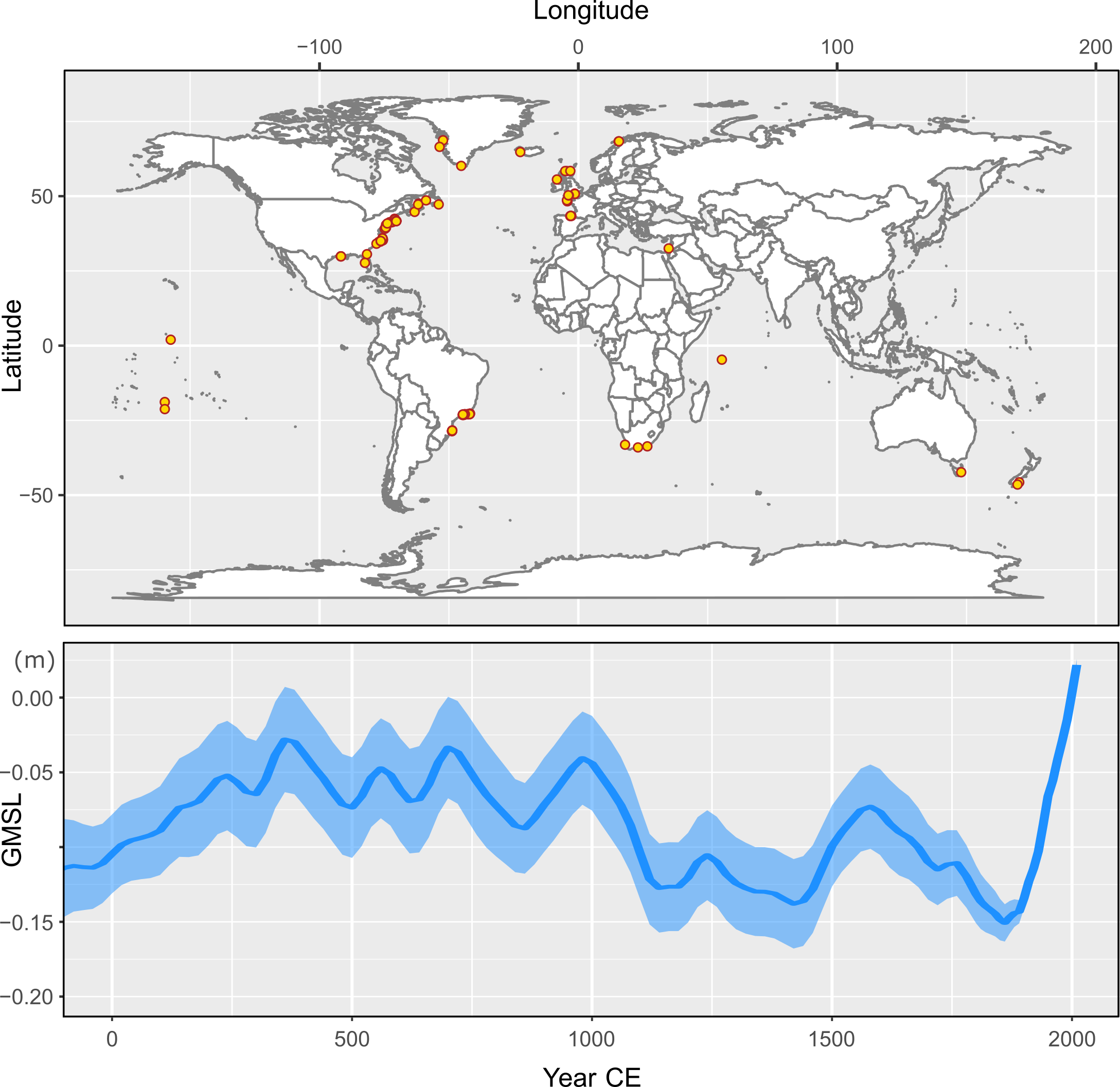 |
|
Figure 1: Location of late Holocene relative sea-level reconstructions (top panel) in the database used to develop the Common Era global mean sea-level curve (bottom panel) of Kopp et al. (2016). |
Calibration of semi-empirical models using the late Holocene GMSL reconstruction of Kopp et al. (2016) and global temperature reconstructions (e.g. PAGES 2k Consortium 2017) is one way in which proxy RSL reconstructions are used to constrain GMSL projections. Temperature projections from Representative Concentration Pathways are used to force the calibrated model and develop GMSL projections. When calibrated only with instrumental data, semi-empirical models often generate higher GMSL projections than process-based models (e.g. Church et al. 2013). However, calibration with late Holocene GMSL and temperature yields similar projections for semi-empirical and process-based models (Kopp et al. 2016). Using these models, Bittermann et al. (2017) explored how GMSL could change under climate scenarios that are compatible with the Paris Agreement.
Regional sea-level changes
Many physical processes that drive late Holocene RSL changes produce distinctive spatial and temporal patterns. Differences and similarities among RSL records can therefore yield insight into the processes that caused late Holocene RSL change. GIA effects include crustal rebound, continental levering, ocean syphoning, and Earth rotational feedbacks from redistribution of mantle and ocean mass (Milne and Mitrovica 1998). Isostatic changes from GIA and sediment- and hydro-(un)loading of the lithosphere cause spatially variable vertical land motion that affects regional RSL signals. RSL changes resulting from Greenland, Antarctic, and glacial meltwater are also spatially variable because of reorganization of the geoid resulting in higher or lower than average RSL rise in the far or near-field respectively (Mitrovica et al. 2001). Late Holocene RSL stability reconstructed from far-field (Indian Ocean) coral microatolls on Kiritimati (Fig. 2) was used to infer minimal ice-ocean mass flux during this period (Woodroffe et al. 2012). Steric (thermal and salinity) changes cause spatially variable sea-surface height changes, although how these signals propagate from the central ocean to the coast remains poorly understood. Ocean and atmosphere circulation modes drive dynamic sea-level variations due to baroclinic gradients causing redistribution of existing ocean mass.
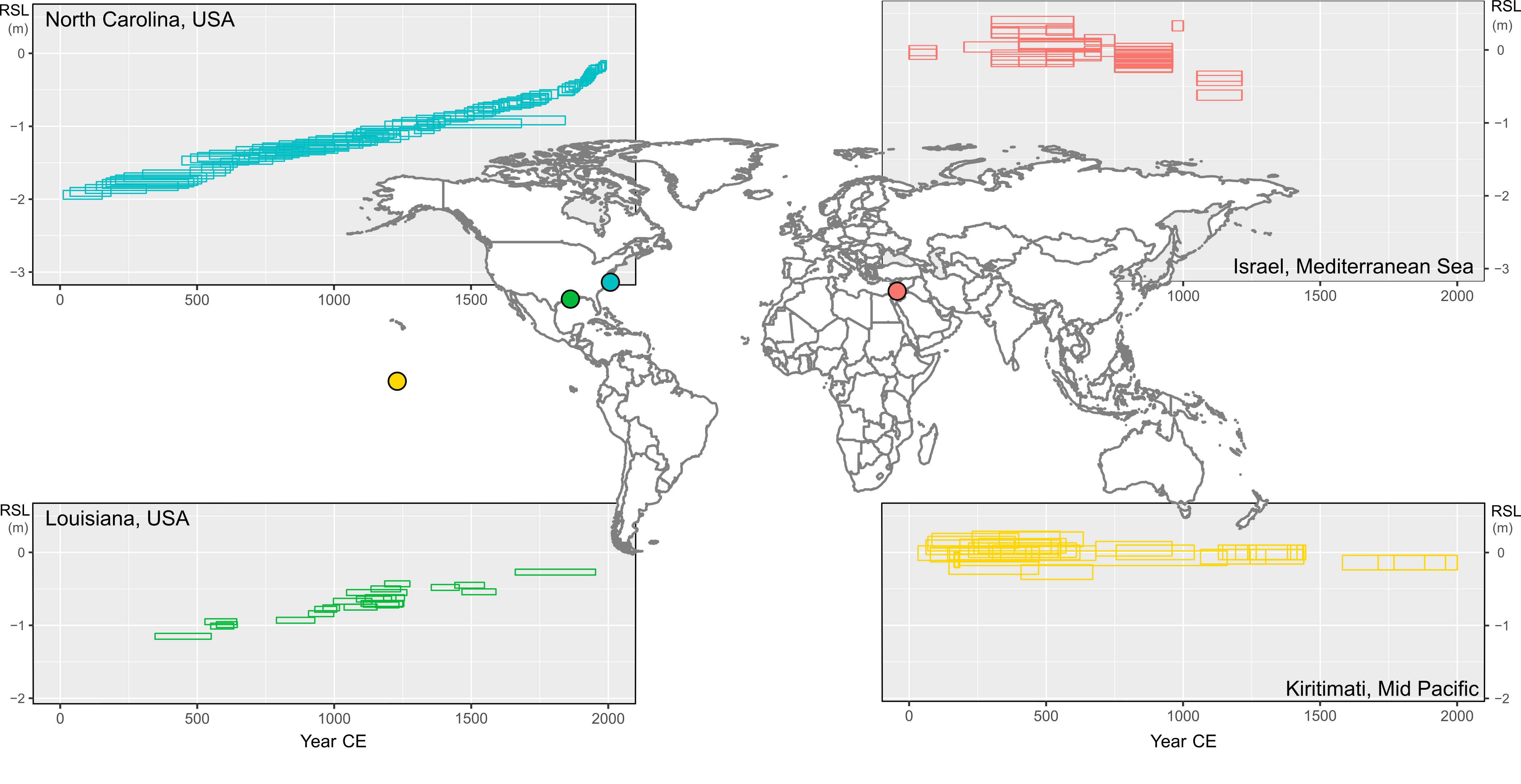 |
|
Figure 2: Selected late Holocene RSL reconstructions developed from salt-marsh sediment (North Carolina; Kemp et al. 2017 and Louisiana; González and Törnqvist 2009), coral microatolls (Kiribati; Woodroffe et al. 2012) and archaeological remains (Israel; Sivan et al. 2004). |
Separation of RSL records into individual driver-related signals remains an active and ongoing challenge. Positive identifications are dependent on a critical spatial density of records so that local-, regional-, and global-scale signals are distinguishable. To date, this density of records only exists in the western North Atlantic Ocean (Fig. 1). Kemp et al. (2018) used a spatio-temporal model to estimate global, regional linear, regional non-linear, and local components of RSL changes with a focus on the western North Atlantic. The analysis resolves GIA effects (the regional linear component) independent from GIA models and identified regional non-linear trends that point to ocean-atmosphere dynamic forcing during the late Holocene. Addressing the spatial distribution bias of RSL records is an important and necessary step towards expanding these spatio-temporal analyses to other regions. A point of emphasis in future work should be replication of RSL reconstructions (within cores, sites and regions) to better differentiate regional RSL signals from possible reconstruction biases and local effects.
affiliations
1Coastal Zone Dynamics and Integrated Management Laboratory, University of Quebec at Rimouski, Canada
2Geography, College of Life and Environmental Sciences, University of Exeter, UK
3Department of Earth and Ocean Sciences, Tufts University, Medford, MA, USA
4Department of Environment and Geography, University of York, UK
contact
Rob Barnett: r.barnettexeter.ac.uk
references
Barlow NLM et al. (2013) Glob Planet Cha 106: 90-110
Bittermann K et al. (2017) Env Res Lett 12: 124010
Church JA et al. (2013) IPCC AR5 WG1: 1137-1216
González JL, Törnqvist TE (2009) Quat Sci Rev 28: 1737-1749
Kemp AC et al. (2015) Curr Clim Cha Rep 1:205-215
Kemp AC et al. (2017) Quat Sci Rev 160:13-30
Kemp AC et al. (2018) Quat Sci Rev 201:89-110
Kopp RE et al. (2016) PNAS 113: 1434-1441
Milne GA, Mitrovica JX (1998) Geophys J Int 133: 1-10
Mitrovica JX et al. (2001) Nature 409: 1026-1029
PAGES 2k Consortium (2017) Sci Data 4: 170088
Shennan I (2015) In: Shennan I et al. (Eds) Handbook for Sea Level Research. Wiley, 3-28
Andrea Dutton1 and Natasha L.M. Barlow2
The Last Interglacial (LIG, Marine Isotope Stage 5e) represents the most recent time period when the polar ice sheets retreated significantly from their present extent, and hence has frequently been cited as a useful, though imperfect, analogue to understand future ice-sheet and sea-level response to a warming climate.
The LIG sea-level highstand that persisted from ~129 to 116 thousand years (kyr) ago has long been acknowledged to be higher than present sea level, though the magnitude of peak sea level and the stability of sea level during the highstand are still actively debated (Dutton et al. 2015a; Austermann et al. 2017; Barlow et al. 2018). While there are important differences between modern, anthropogenically-driven global warming and the orbitally driven warmth of the LIG, there are several relevant and valuable observations to be made. Among these are (1) understanding the sensitivities of the ice sheets in Greenland and Antarctic to warming; (2) identifying the mechanisms contributing to the millennial-scale evolution of climate and sea level during the interglacial; and (3) mapping out the sea-level budget, including the sources, magnitudes, and timing of meltwater contributions. Fundamentally, one of the most critical questions to answer is whether there was a significant contribution from the Antarctic ice sheet to LIG sea level, which is still uncertain.
Magnitude of peak LIG sea level
Sea level varies geographically, due to a combination of processes including glacial isostatic adjustment (GIA) and dynamic topography (Milne et al. this issue; Austermann and Forte, this issue). Therefore, the maximum height of LIG sea level will not be the same at every location or occur at the same time (Dutton and Lambeck 2012). Several research groups have independently assessed peak global mean sea level (GMSL) from a combination of individual observations of relative sea level from globally distributed localities (Kopp et al. 2009; Dutton and Lambeck 2012; Düsterhus et al. 2016) (Fig. 1). Though these estimates vary somewhat from each other, GIA-corrected reconstructions for GMSL appear to converge on values of ~6-9 m above present for the peak of LIG sea-level rise. An important qualification to this interpreted range is the recognition that vertical motion of the earth’s surface due to mantle convection (dynamic topography) since the LIG could easily be on the order of a few meters – up or down – depending on the location (Austermann et al. 2017). While this casts additional uncertainty on the provisional ~6-9 m estimate, it is not straightforward to provide either accurate or precise assessments of the magnitude of the dynamic topography signal for specific sites, and hence difficult to determine if and how this estimate of peak sea level should be further modified.
 |
|
Figure 1: Estimates of global mean sea-level highstand during the Last Interglacial compared to today. All studies correct for glacial isostatic adjustment. |
Sources of LIG sea-level rise
There is evidence from both observations and models that the Greenland ice sheet was significantly smaller than present during the LIG. Though the summary of several studies presented by Dutton et al. (2015a) indicated a convergence towards 2 m (± 1.5) of GMSL contribution from Greenland, a subsequent modeling study increased this estimate to 5.1 m (4.1 to 6.2, 95% credible interval; Yau et al. 2016). To some extent, the disagreement between studies in terms of inferred ice-sheet size may be due to the conflicting implications of total gas content in the ice cores versus temperature estimates. Nonetheless, ice-sheet models consistently produce a couple meters or more of sea-level rise coming from Greenland, with peak contributions at ~121-122 kyr before present. In the absence of near-field data for Antarctica, estimates for an Antarctic contribution to LIG GMSL have typically been calculated by subtracting the contributions of other sources (Greenland, thermal expansion, and mountain glaciers) from far-field sea-level estimates. Given the large unknowns that exist in both peak GMSL and the Greenland ice-sheet contribution, this approach does not allow us to definitively determine whether a sector of the Antarctic ice sheet collapsed during the LIG. However, based on sediment provenance from circum-Antarctic cores, or estimates of sufficiently high GMSL early in the LIG (prior to significant retreat in Greenland), some have argued for a smaller Antarctic ice sheet compared to present at some point during the LIG (Dutton et al. 2015b; Wilson et al. 2018). Confidently “fingerprinting” a few meters of GMSL contribution from either Greenland or Antarctica by using the expected patterns in spatial variability of relative sea level due to GIA to identify the timing and sources of meltwater contribution is a provocative idea. However, this approach would require decimeter-scale vertical precision, which is typically well within the uncertainties of geologic sea-level indicators, hence making the fingerprint of individual ice sheets difficult to carry out in practice.
Evolution of the sea-level highstand
The sea-level highstand has been variously reported to have had anywhere from one to four peaks, where multiple peaks define millennial-scale fluctuations in sea level. Some reconstructions simply connect age-elevation data points from corals with a line, which ignores potential changes in coral paleowater depths and contextual sedimentary and stratigraphic information from fossil reef outcrops. While the coral age-elevation-taxonomy compilation by Hibbert et al. (2016) drives the point home that paleowater depth ranges of corals can be large, this does not render the entire fossil coral archive useless for addressing the question of whether there were sea-level oscillations during the LIG. Instead, sedimentary evidence for changes in water depth, including intervals of subaerial exposure within the fossil reef or evidence of rapid reef accretion, can be used to more confidently interpret possible meter-scale changes. In fact, several studies have pointed to compelling evidence for abrupt changes in sea level preserved in LIG reef sequences (e.g. Blanchon et al. 2009; Skrivanek et al. 2018). The magnitude of these changes is poorly constrained, however. To confidently confirm these rapid sea-level changes at a global scale, more evidence needs to be amassed from geographically diverse sites with robust chronologies. Some recent studies have argued that a sea-level fall of >4 m, as indicated by Kopp et al. (2009), is not plausible given constraints from phreatic overgrowths in Mallorca caves (Polyak et al. 2018) and other lines of observational and modeling evidence (Barlow et al. 2018). However, these studies do not preclude the possibility of smaller, meter-scale sea-level fluctuation(s) in the low latitude reef sites during the LIG (Fig. 2).
 |
|
Figure 2: Field evidence from LIG sequences in (A) The Bahamas (Skrivanek et al. 2018) and (B) Seychelles (Vyverberg et al. 2018) that is consistent with an ephemeral sea-level fall occurring between the development of stratigraphically distinct reef units. Depending on the site, truncated corals in the lower reef, extensive dissolution on the reef surface, or sequence of freshwater and marine cements provide evidence of an ephemeral sea-level fall. |
Implications for links between climate, ice sheets, and sea level
There is great interest within the community to move beyond the big-picture view of the correspondence between peak temperatures and peak GMSL during the LIG, for example as depicted in Dutton et al. (2015a). Increasing attention is being drawn to millennial-scale changes in temperature, ice-sheet response, and the accompanying changes in sea level during the LIG to understand the thresholds for ice-sheet collapse, the temporal relation between climate forcing and sea level, and the rates of sea-level change. One of the biggest challenges in linking climate signals to observations of sea-level change is developing accurate, precise, and highly resolved chronologies that can confidently be correlated to other records, for instance, between data from deep-sea cores and U-Th dated archives of sea-level change in coral reefs. Tzedakis et al. (2018) demonstrate that climate in the North Atlantic region was more variable during the LIG than the Holocene, but it is yet to be firmly established how that variability links to concomitant changes in ice volume, meltwater input and sea level.
What is clear, however, is that the more we can extract from the paleo record about the phasing, magnitude, and sources of meltwater input into the oceans, the better we can constrain the models that are used to project future sea-level rise. We envision that interdisciplinary approaches to this question will be essential to unravelling the dynamics of shrinking polar ice sheets in a warming world.
affiliations
1Department of Geological Sciences, University of Florida, Gainesville, USA
2School of Earth and Environment, University of Leeds, UK
contact
Andrea Dutton: aduttonufl.edu
references
Austermann J et al. (2017) Sci Adv 3: e1700457
Barlow NLM et al. (2018) Nat Geosci 11: 627-634
Blanchon P et al. (2009) Nature 458: 881-884
Düsterhus A et al. (2016) Geophys J Int 206: 900-920
Dutton A, Lambeck K (2012) Science 337: 216-219
Dutton A et al. (2015a) Science 349: aaa4019
Dutton A et al. (2015b) Quat Sci Rev 107: 182-196
Hibbert FD et al. (2016) Quat Sci Rev 145: 1-56
Kopp RE et al. (2009) Nature 462: 863-867
Polyak VJ et al. (2018) Nat Geosci 11: 860-864
Skrivanek A et al. (2018) Quat Sci Rev 200: 160-177
Tzedakis PC et al. (2018) Nat Commun 9: 4235
Vyverberg K et al. (2018) Mar Geol 399: 170-187