PAGES Magazine articles
Amy Leventer1, K.E. Kohfeld2, C.S. Allen3, X. Crosta4, A. Marzocchi5, J. Prebble6 and R.H. Rhodes7
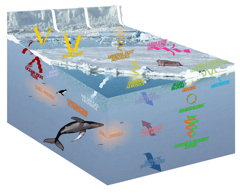
Sea ice is a critical component of the climate system (Fig. 1), influencing heat and gas exchange between the atmosphere and polar oceans. Given the high albedo of sea ice relative to that of open water, seasonal variability in sea-ice extent impacts reflectivity of the Earth's surface. Changes in the Antarctic sea-ice seasonal cycle also affect Southern Ocean water mass buoyancy, thereby modulating Southern Ocean upper and lower overturning cells and global ocean circulation. Through its interactions with the glacial ice margin, sea ice affects, and is affected by, ice sheets and ice shelves. Finally, sea-ice decay impacts ocean primary productivity through its roles in seeding phytoplankton and driving upper-ocean stratification and nutrient distribution (e.g. Armand et al. 2017). At present, average Antarctic sea-ice extent ranges between summer minima of ~3 million km2 to winter maxima of ~18 million km2 (Cavalieri and Parkinson 2008). Changes in sea-ice extent over longer time periods have been studied since the late 1970s. Community-based research efforts have focused on understanding different sea-ice proxies (e.g. the PAGES Sea Ice Proxies working group), and on reconstructing Antarctic sea-ice extent for specific time periods, such as the Last Glacial Maximum through the project MARGO (Multiproxy Approach for the Reconstruction of the Glacial Ocean Surface; Gersonde et al. 2005).
 |
|
Figure 1: Principal feedbacks and interactions between Antarctic sea ice and the ocean, biosphere, atmosphere, and cryosphere (reproduced from Patterson et al. 2019). |
The C-SIDE working group (pastglobalchanges.org/c-side) was established to extend Southern Ocean sea-ice reconstructions back further in time, with a focus on the past 130,000 years. This longer timescale allows us to evaluate the role of sea ice on major climate transitions including the glacial inception, when carbon was sequestered in the ocean, and deglaciation, when ocean carbon reserves were released into the atmosphere. This time frame also encompasses the penultimate interglacial when Antarctica was ~2ºC warmer than today – a useful "process" analogue for future warming scenarios. The main difference between C-SIDE and previous large-scale projects (MARGO) is that C-SIDE aims to document sea-ice dynamics along with understanding processes and interactions between Antarctic sea ice and global climate on different timescales. In addition, C-SIDE aims to include these data in Earth system modeling efforts, including the Paleoclimate Modelling Intercomparison Project (pmip3.lsce.ipsl.fr).
Our first C-SIDE workshop was held from 24-26 October 2018 in Vancouver, Canada (Patterson et al. 2019; doi.org/10.22498/pages.27.1.31). Major accomplishments included developing a format for compiling proxy datasets from both marine-sediment and ice-core records, establishing an initial inventory of 170 sites with potential information on sea-ice changes, and assigning data-mining efforts to be completed before the next workshop. These tasks are critical as we seek to provide denser spatial coverage and higher temporal resolution of sea-ice variability through time.
Our second workshop, "Sea-ice database and model-data framework" (https://doi.org/10.22498/pages.27.2.86), was held 29-31 August 2019 in Sydney, Australia, immediately prior to the 13th International Conference on Paleoceanography (pastglobalchanges.org/calendar/128542). The primary goal was to complete our inventory of paleo records, with details about the temporal extent of each published, unpublished, and future targeted record, as well as the data type used to reconstruct sea ice. These include, but are not limited to, diatom assemblages, organic biomarkers such as highly branched isoprenoids, isotopic evidence, and geochemical data from ice cores. Our database will be completed by entering sea-ice records that allow for examination of full time series as well as spatial patterns associated with specific time intervals, including the Holocene, the last 40 kyr, MIS 5, and the last 130 kyr. Ultimately, our plan is to target regional transects, extending from ice sheets to the equatorward extent of sea ice. We recognize that, at this time, only a limited number of datasets extend back 130,000 years, with even fewer that span latitudinal transects. However, identification of the data gaps is critical for the establishment of new priorities for future field-based data collection.
Affiliations
1Department of Geology, Colgate University, Hamilton, NY, USA
2School of Resource and Environmental Management, Simon Fraser University, Burnaby, BC, Canada
3British Antarctic Survey, Cambridge, UK
4University of Bordeaux, France
5National Oceanography Centre, Southampton, UK
6GNS Science, Lower Hutt, New Zealand
7Department of Geography and Environmental Sciences, Northumbria University, Newcastle-upon-Tyne, UK
contact
Karen Kohfeld: kohfeld sfu.ca
references
Cavalieri DJ, Parkinson CL (2008) J Geophys Res Oceans 113: C07004
Maija Heikkilä1, A. Pieńkowskiv2, S. Ribeiro3 and K. Weckström1
The Arctic cryosphere is transforming rapidly in response to recent climate change. Accelerated melt of glaciers, ice caps and the Greenland ice sheet, increased glacial runoff, diminishing sea-ice extent and volume, coastal erosion, and permafrost thaw all have profound impacts on Arctic coastal environments (Fig. 1). The fjords and other nearshore areas form a productive zone that is vital to both Arctic biodiversity and the subsistence of local communities. Increased inputs of freshwater and sediments from land, together with diminishing sea-ice cover, will have a critical effect on future biogeochemical cycling, primary production, and key ecosystem services in the coastal zone.
 |
|
Figure 1: Cryosphere changes both on sea and on land have a profound influence on coastal marine ecosystems in the Arctic. |
Recent studies show that the impacts of land-derived freshwater on coastal circulation and contributions of dissolved and particulate matter are heavily dependent on the marine system, and have a non-linear impact on primary productivity (Hopwood et al. 2018). For example, marine-terminating glaciers induce nearshore nutrient upwelling and hence primary production, while fjords fed by land-terminating glaciers are low-production zones often characterized by a light-limiting layer of suspended matter (Meire et al. 2017). Furthermore, the coastal zone interacts dynamically with the open ocean. Land-derived meltwater can affect primary production far away from the coastal zone (Arrigo et al. 2017), while waters transported by large-scale current systems have an influence on the hydrography of some coastal systems (Sejr et al. 2017).
A major challenge facing arctic marine scientists today is the paucity of reference ecological data from which to interpret recent and future changes. Many proxy methods have been proposed based on microfossil, biogeochemical, and to some extent molecular records of sympagic, planktic, and benthic organisms to reconstruct past marine ecosystem changes. In particular, deciphering past sea-ice concentrations (de Vernal et al. 2013), sea-surface temperatures (e.g. Caissie et al. 2010), and changes in ocean circulation (Rahmstorf 2002) have attracted attention, as they are tightly linked to global paleoclimate changes. However, the multi-faceted nature of coastal ecosystems necessitates consideration of regional- and local-scale influence of cryosphere changes, and their fingerprints in biological and biogeochemical proxy records. Clearly, there is a need for closer cooperation between different proxy specialists and for critical assessment of the current analytical, numerical, and ecological knowledge.
The ACME working group was launched in July 2019, with the aim to assess and refine available marine proxies that can be used to reconstruct past cryosphere changes and their ecosystem impacts in the Arctic coastal zone. A particular focus is placed on the techniques and the quality of data, on the training of early-career scientists, and on the establishment of new community-driven protocols.
ACME is envisioned to run over two three-year phases. The main product goal of Phase 1 (2019-2022) is a database that contains a spatial network of currently available sites and proxies commonly used for reconstructing sea ice, primary production, meltwater runoff and terrestrial inputs in Arctic coastal and fjord environments. Each database entry will follow the criteria defined by the ACME community in the early stages of Phase 1. This will ensure that quality assessment of database entries will be easy for the end users. Furthermore, ACME seeks to facilitate community integration by promoting knowledge transfer and collaboration among proxy specialists, and knowledge integration of the paleo and monitoring communities. Importantly, ACME fosters critical, methodological understanding and data handling skills of the next generation of paleoceanographers and paleoenvironmental researchers.
From 17 October to 15 November 2019, ACME conducted a survey to collect community perspectives on the current state and future directions of Arctic coastal paleoceanography. The results of the survey will provide a basis for outlining priority research questions and community directions, and give an overview of spatial, methodological, and ecological knowledge gaps identified by the community.
The ACME community will meet during the first workshop to plan the database structure and proxy-specific data entry criteria at the EGU General Assembly from 3-8 May 2020 in Vienna, Austria. For more information about this working group, see the ACME website (pastglobalchanges.org/acme), sign up for the ACME mailing list (listserv.unibe.ch/mailman/listinfo/acme.pages), and follow ACME on Twitter (@AcmePages).
affiliations
1Environmental Change Research Unit (ECRU), Ecosystems and Environment Research Programme, University of Helsinki, Finland
2Norwegian Polar Institute, Tromsø, Norway
3Department of Glaciology and Climate, Geological Survey of Denmark and Greenland (GEUS), Copenhagen, Denmark
contact
Maija Heikkilä: maija.heikkilahelsinki.fi
references
Arrigo KR et al. (2017) Geophys Res Lett 44: 6278-6285
Caissie BE et al. (2010) Paleoceanography 25: PA1206
de Vernal A et al. (2013) Quat Sci Rev 79: 1-8
Hopwood MJ et al. (2018) Nat Comm 9: 3256
Meire L et al. (2017) Global Change Biol 23: 5344-5357
Donald E. Penman1 and Sandra Kirtland Turner2
The Paleocene-Eocene Thermal Maximum (PETM, 56 Myr BP) was a rapid greenhouse-gas-driven global warming event highlighted for comparison to anthropogenic climate change. Proxies and modeling indicate that changing patterns of global overturning circulation overprinted paleoceanographic records of this event.
In 1991, Kennett and Stott published a groundbreaking record of the carbon and oxygen isotope composition of foraminifera from Southern Ocean deep-sea sediments spanning the Paleocene-Eocene boundary. They observed striking negative excursions in both isotopic systems, unlike any rapid shifts known from the paleoceanographic record, coincident with the largest benthic extinction of the Cenozoic. The oxygen isotopes indicated a sudden warming of both surface and deep Antarctic waters, while the carbon isotope excursions (CIE) suggested a collapse in vertical δ13C gradients. Those authors concluded that changes in the global overturning circulation must be the cause of these unusual paleoceanographic observations and the extinction – but a proliferation of coeval sedimentary records in the decades since has transformed this interpretation.
From local findings to global observations
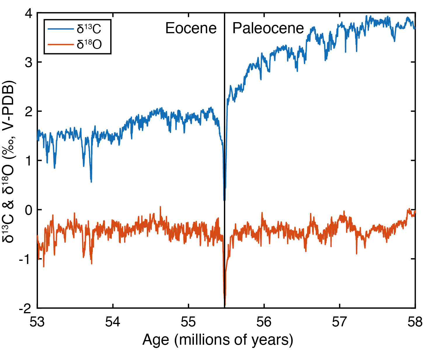
The CIE and warming first recognized in the Southern Ocean have now been observed globally from both the marine and terrestrial realms (Fig. 1; see e.g. McInerney and Wing 2011 for a compilation), in organic and inorganic carbon, and coincide with evidence for global ocean acidification (Babila et al. 2018; Zachos et al. 2005), large reorganizations of the hydrologic cycle (Wing et al. 2005; Zachos et al. 2003), and biotic turnover both on land and in the sea (Speijer et al. 2012). The modern interpretation holds that this event (now known as the Paleocene-Eocene Thermal Maximum or PETM) was driven by the geologically rapid (within thousands of years) addition of a large mass (thousands of gigatons) of isotopically light carbon into the atmosphere and ocean. Without the global coverage provided by more recent observations, Kennett and Stott did not know what triggered their proposed change in circulation, but in a sense their interpretation still holds: marine records of the PETM reflect not only global carbon cycle processes, but also the regional effects imparted by the changes in ocean circulation that we still think occurred during the PETM.
 |
|
Figure 1: Bulk-sediment carbon and oxygen isotope stratigraphy of Site 1262 from the late Paleocene through the early Eocene (Zachos et al. 2010). The large negative excursions in both isotope systems at the Paleocene-Eocene boundary represents the PETM. |
Basinal asymmetry in pelagic PETM sedimentary records
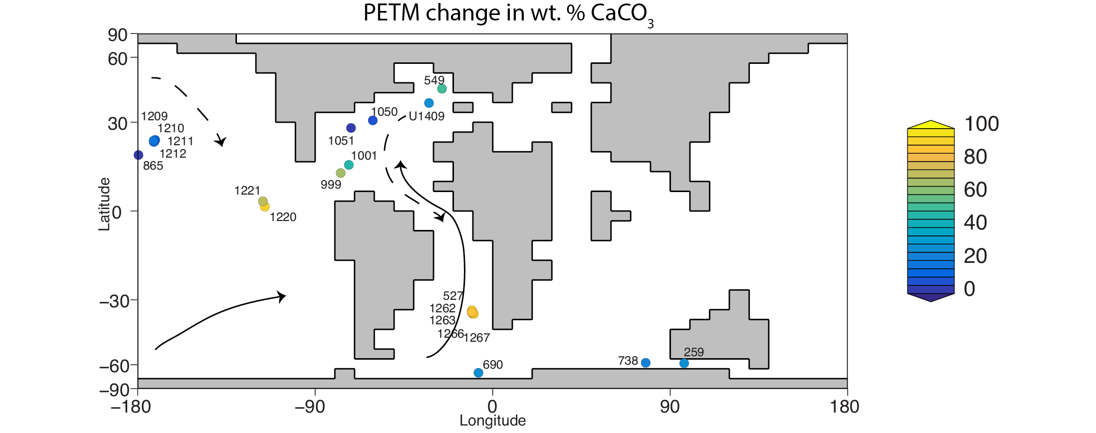
Comparison of PETM deep-sea records reveals several regional differences in lithology and geochemistry that illustrate the profound influence of changing ocean circulation during the event. CaCO3 dissolution is a hallmark of pelagic PETM records, characterized by a temporary decline or absence of the calcareous microfossils that typically constitute pelagic sediments, resulting in a conspicuous clay layer. This dissolution is an expected consequence of CO2 addition to seawater, which lowers pH and carbonate saturation state (Ω) in tandem. Paleoceanographers often quantify the extent of dissolution by reconstructing the shoaling of the carbonate compensation depth (CCD), the "snowline" of the ocean below which carbonates are absent from sediments. However, there are significant regional differences in the extent of PETM CaCO3 dissolution (or the existence and thickness of clay layers). In the South Atlantic, PETM clay layers identified from a depth transect of ocean drilling sites indicate that the CCD shoaled by greater than 2 km and suggest the dissolution of CaCO3 over huge regions of the seafloor (Zachos et al. 2005). In contrast, a similar depth transect in the subtropical North Pacific shows comparatively limited CaCO3 dissolution, constraining the CCD shoaling in that basin to less than 0.5 km (Colosimo et al. 2005; Zeebe and Zachos 2007). Much of this basinal asymmetry can be explained by a reorganization of deep-sea circulation. Deep water becomes more corrosive to CaCO3 (lower Ω) with age due to the accumulation of respired organic carbon, such that the modern CCD in the deep North Pacific (filled with the ocean's oldest seawater) is ~1 km deeper than in the North Atlantic (which, as a region of deep-water formation, contains the youngest deep water). Using a sediment model forced with records of varying CaCO3 weight percentages (wt. %) at different globally distributed pelagic sites, Zeebe and Zachos (2007) determined that CaCO3 undersaturation at the peak of the PETM was more severe in the Atlantic than in the Pacific – the opposite of the modern pattern. Those authors concluded that deep-water circulation patterns must have been reversed (relative to the modern configuration) during the acidification phase of the PETM. This idea was expanded upon by the PETM carbon-cycle simulation of Zeebe et al. (2009), who implemented a transient shift in the locus of deep-water formation from the Southern Ocean to the North Pacific.
 |
|
Figure 2: Change in pelagic sedimentary wt. % CaCO3 over the PETM (colored circles) plotted on the cGENIE model Paleocene land mask (Panchuk et al. 2008). Data were compiled from Zeebe and Zachos (2007) and Panchuk et al. (2008), but see references therein for original records. Arrows show inferred circulation for pre-event (solid lines) and PETM (dashed lines) based on changing δ13C gradients and basinal asymmetry in CaCO3 dissolution. |
Disparate benthic CIE magnitudes
Another hallmark of the PETM that is susceptible to overprinting by changing ocean circulation is the size of the benthic foraminiferal CIE, which varies significantly from site to site (McInerney and Wing 2011; Nunes and Norris 2006). In theory, the benthic CIE due to a rapid carbon release should simply reflect the mass and δ13C of the carbon input, and be relatively homogenous throughout the deep sea, given that typically low pelagic sedimentation rates are unlikely to resolve differences on timescales shorter than ocean mixing (1-2 kyr). The δ13C of dissolved carbon in deep seawater decreases as it ages due to the accumulation of isotopically light respired organic carbon. In the modern ocean, this leads to a 1‰ δ13C difference between young North Atlantic deep water and old North Pacific deep water. Deep-water circulation is hence a powerful lever on regional benthic δ13C – an abrupt reversal of the modern deep-water aging gradient would force Pacific benthic δ13C 1‰ heavier and Atlantic δ13C 1‰ lighter in the long term. An abrupt reorganization of deep-water circulation patterns at the PETM onset could similarly help explain the range of deep-ocean benthic foraminiferal CIE sizes observed globally, which span 0.5‰ to 3.5‰ (McInerney and Wing 2011). Nunes and Norris (2006) produced a global compilation of deep-ocean benthic CIE records and argued that the generally smaller CIE magnitude in the Northern Hemisphere compared to the Southern Hemisphere resulted from a switch in the locus of deep-water formation from the Southern Ocean to the North Atlantic. Additional complications remain, including truncation of the base of the event due to carbonate dissolution at some sites (leading to an apparently smaller CIE) and the role of bioturbation (mixing by benthic organisms) but changing ocean circulation patterns are clearly a factor in the disparate magnitude of benthic CIEs.
Additional geochemical indicators
While deep-sea records of CaCO3 wt. % and δ13C are most common, there is evidence for ocean circulation impacting other PETM geochemical records as well. Proxies for deep-ocean oxygen (Pälike et al. 2014) and patterns of silica burial (Penman et al. 2019) indicate asymmetry between the Atlantic and Pacific basins during the PETM. Neodymium isotopes, a quasi-conservative tracer of ocean circulation, may even more directly indicate changes in deep-ocean ventilation associated with shifting patterns of overturning circulation (Abbott et al. 2016; Blaser et al. this issue).
Mechanisms for PETM circulation change from ocean-physics models
Sedimentological evidence suggests that a change in deep-ocean circulation was likely during the PETM, and physical models provide possible causal mechanisms. Using a model of ocean physics forced offline by an atmospheric general circulation model, Bice and Marotzke (2002) explored the role that the hydrologic cycle might have played in linking global warming to changes in ocean circulation at the PETM. With warming, the hydrologic cycle intensifies, transporting more water vapor from low to high latitudes. This increases the poleward latent heat flux and redistributes evaporation and precipitation globally, changing patterns of sea-surface salinity. Both of these (heat and freshwater transport) change the density gradients of surface seawater, which makes surface waters in different regions of the ocean more or less susceptible to sink and form deep water. Bice and Marotzke’s experiments favored a switch from Southern to Northern Hemisphere deep-water formation during peak PETM forcing, broadly consistent with the hypotheses proposed by Zeebe et al. (2009) and Nunes and Norris (2006), but the exact locus and flux of northern deep-water formation is sensitive to uncertain paleogeography and is still debated. Numerical modeling of an instantaneous warming event simulated with the UVic Earth system model of intermediate complexity by Alexander et al. (2015) provides a consistent and more detailed scenario in which corrosive North Atlantic bottom water spills into the South Atlantic with the onset of North Atlantic deep-water formation over the several thousand years following instantaneous CO2 release.
Together, modeling and geochemical study of the PETM demonstrate that it is crucial to consider changes in the global overturning circulation, and not just global carbon cycle processes, in the interpretation of sedimentary records of ancient climate perturbations.
affiliations
1Geology and Geophysics, Yale University, New Haven, CT, USA
2Department of Earth Science, University of California Riverside, USA
contact
Donald E. Penman: donald.penmanyale.edu
references
Abbott AN et al. (2016) Clim Past 12: 837-847
Alexander K et al. (2015) Nat Geosci 8: 458-461
Babila T et al. (2018) Philos T R Soc A 376: 20170072
Bice KL, Marotzke J (2002) Paleoceanography 17: 1018
Kennett JP, Stott LD (1991) Nature 353: 225-229
McInerney FA, Wing SL (2011) Annu Rev Earth Pl Sc 39: 489-516
Nunes F, Norris RD (2006) Nature 439: 60-63
Pälike C et al. (2014) Geochem Geophy Geosy 15: 1038-1053
Panchuk K et al. (2008) Geology 36: 315-318
Penman DE et al. (2019) Paleoceanogr Paleocl 34: 287-299
Speijer R et al. (2012) Austrian J Earth Sci 105: 6-16
Wing SL et al. (2005) Science 310: 993-996
Zachos JC et al. (2003) Science 302: 1551-1554
Zachos JC et al. (2005) Science 308: 1611-1615
Zachos JC et al. (2010) Earth Planet Sc Lett 299: 242-249
Pinxian Wang and Jun Tian
The 400-kyr eccentricity cycles dominate marine δ13C records until 1.6 Myr BP, coeval with the final formation of an abyssal carbon reservoir in the Southern Ocean. Eccentricity-driven global monsoon cycles are hypothetically responsible for this 400-kyr rhythm, which could have been further influenced by oceanographic processes related to polar ice-sheet growth.
According to Milankovitch theory, Earth's eccentricity has periods of 100 and 400 thousand years (kyr). Therefore, a long eccentricity cycle (400 kyr) should be embedded in paleoclimate records. The absence of such a signal puzzled the paleoclimate community 30 years ago and was considered a fundamental problem in paleoclimate research ("the 400-kyr problem"). Recently, an increasing number of proxy records have revealed the existence of these 400-kyr cycles, at least in many records from the Cenozoic and Mesozoic (e.g. Giorgioni et al. 2012; Kocken et al. 2019). The remarkable 400-kyr eccentricity signal in deep-sea records now is referred to as the "heartbeat" of the ocean system (Pälike et al. 2006), and is used for astronomical calibration of the Cenozoic, Mesozoic, and beyond.
Complexity of the 400-kyr δ13C signal
Because of the long residence time of carbon in the oceanic reservoir greater than 100 kyr, the long eccentricity cycle is best documented in the deep-sea δ13C records, with maximum values (δ13Cmax) occurring at eccentricity minima. This δ13C oscillation reflects periodic changes in the sources and sinks of oceanic and atmospheric carbon, likely driven by the global monsoon. However, the mechanism remains unclear (Wang et al. 2017). The "rain-ratio hypothesis", for example, ascribed these δ13C cycles to the ratio of organic versus inorganic carbon deposition in the deep ocean, which is dominated by the ratio of diatoms to coccoliths (Archer et al. 2000). However, this was challenged by the discovery of the "ballast mineral" effect, as silicate and carbonate biominerals can affect deep-water flux of organic carbon (Armstrong et al. 2001). By contrast, the dissolved organic carbon (DOC) hypothesis (Wang et al. 2014) attributes the δ13C changes to the ratio between particulate and dissolved organic carbon (POC/DOC) in the ocean, which in turn depends on the monsoon-controlled nutrient supply. This DOC hypothesis was based on the recently identified microbial carbon pump (MCP) in the ocean (Jiao et al. 2010) and supported by numerical modeling (Ma et al. 2014).
 |
|
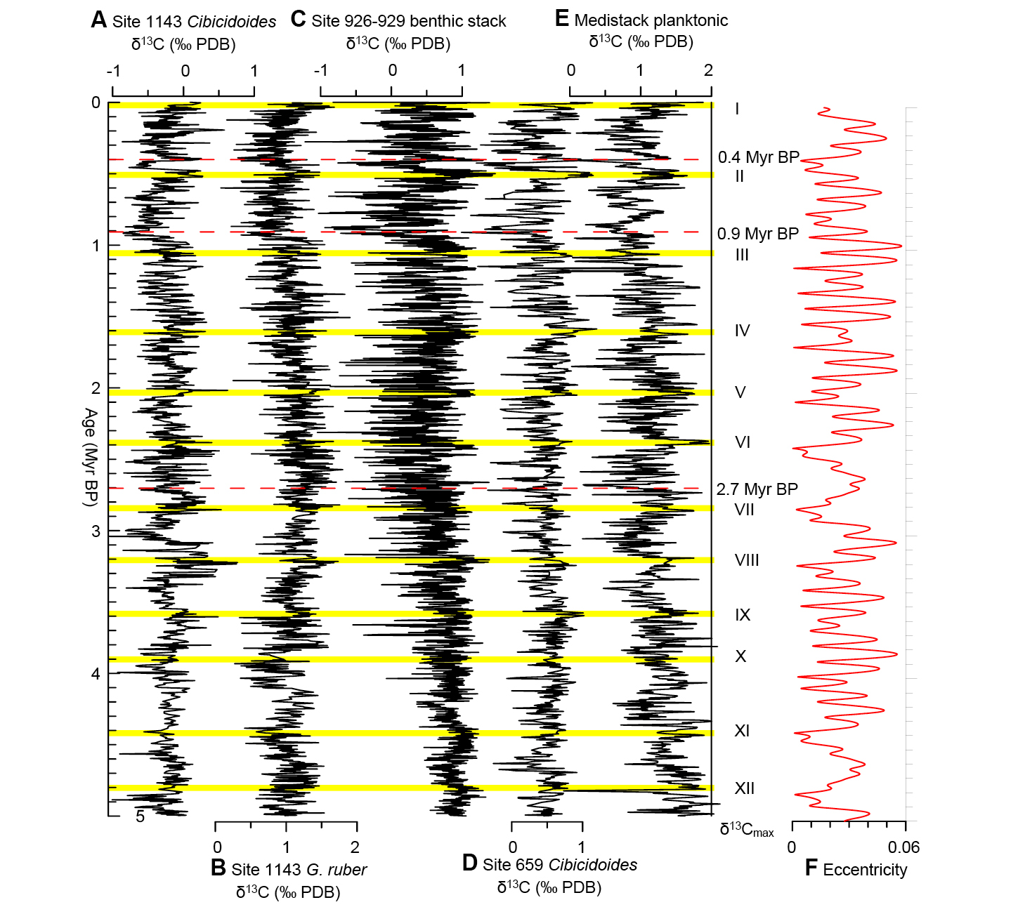
Figure 1: Carbon isotopic records from various oceans over the past 5 Myr (A), (B) ODP Site 1143, South China Sea; (C), (D) Atlantic; (E) Mediterranean stack; (F) Eccentricity. Yellow bars indicate the δ13Cmax events (modified from Wang et al. 2014). |
The hypothesis discussed above does not account for the signal observed in δ13C records from the Quaternary. As displayed in Figure 1, the 400-kyr signal is clear in all δ13C timeseries from various oceans during the Pliocene, and a total of 13 δ13Cmax events corresponding to long eccentricity minima have been identified (Wang et al. 2010). For the Quaternary, however, the rhythmic beat of δ13Cmax at long eccentricity minima ended at 1.6 million years before present (Myr BP), and the following δ13Cmax events were out of phase with the minimum eccentricity signal; the records rather show a 500-kyr cycle over the last million years (Fig. 1). It remains unclear why the long eccentricity cycles disappeared in the Quaternary.
Polar glaciation, Southern Ocean, and the 400-kyr cycles
As shown by spectral analysis, the 400-kyr eccentricity signal in δ13C records became obscured after 1.6 Myr BP at all open-ocean sites but not in the Mediterranean Sea, which has been largely isolated from the global ocean since the late Miocene (Fig. 1e). Accordingly, the disappearance of the 400-kyr cyclicity around 1.6 Myr BP might be attributed to the restructuring of the global ocean, which disturbed responses of the oceanic carbon reservoir to the long eccentricity cycle. This in particular refers to formation of an abyssal carbon reservoir in the Southern Ocean (SO), which began 1.6 Myr BP. Stratification of the polar water column started to drive vertical thermal stratification between deep and intermediate waters in the SO around 2.7 Myr BP, isolating its abyss from the intermediate ocean and finally generating the largest carbon reservoir in the global ocean since 1.6 Myr BP (Hodell and Venz-Curtis 2006).
Since then, the ocean circulation has been divided into an actively circulating upper branch and a sluggish abyssal branch in the SO. As the restructuring of the ocean was accompanied by the growth of polar ice sheets, it is plausible that global glaciation modulates responses of oceanic carbon cycles to the orbital forcing. This is supported by empirical evidence showing that the long eccentricity signal in the marine δ13C records starts to vanish at 1.6 Myr BP (Wang et al. 2014). It is possible that mechanisms of polar ice-sheet growth disturbing the long-term carbon cyclicity show parallels to some climate events in the Miocene. For example, the eccentricity-forced δ13C signal was temporarily obscured around 13.9 Myr BP, presumably as a consequence of the amplification of the Antarctic ice sheet (Holbourn et al. 2007; Tian et al. 2014).
Clearly, the oceanic δ13C oscillation on a 105-year timescale is controlled by both astronomical and oceanographic factors. Astronomically, the oceanic carbon reservoir responds to changes in the POC/DOC ratio, which result from changes in the monsoon-driven nutrient supply. Oceanographically, the abyssal carbon reservoir in the SO might modulate the DOC distribution in the ocean by high-latitude processes associated with ice-sheet growth and decay. As a result, the oceanic δ13C signal is dominated by a regular 400-kyr beat when the low-latitude processes prevail, such as in the ice-free Hot-House world (Miller et al. 1991). In the Ice-House world, on the other hand, the 400-kyr rhythm in the δ13C sequence can be obscured by processes associated with ice-sheet development. This may provide an explanation for the observed disappearance of 400-kyr δ13C cycles in the Quaternary after 1.6 Myr BP.
400-kyr δ13C cycles and Quaternary climate transitions
Changes in the long-term cyclicity of the oceanic carbon reservoir may have serious climatic consequences. Two such changes occurred during the last million-year period, namely the mid-Pleistocene transition (MPT) centered at 0.9 Myr BP and the mid-Brunhes event (MBE) around 0.4 Myr BP. Importantly, both were preceded by δ13Cmax events: the MPT by δ13Cmax-III (~1.0 Myr BP), and the MBE by δ13Cmax-II (~0.5 Myr BP) (Fig. 1; Wang et al. 2004). This indicates that changes in the oceanic carbon reservoir might be strong enough to cause such a major climatic shift during glacial periods. If so, the next step is to determine the potential driving mechanisms and the role of the Southern Ocean.
 |
|
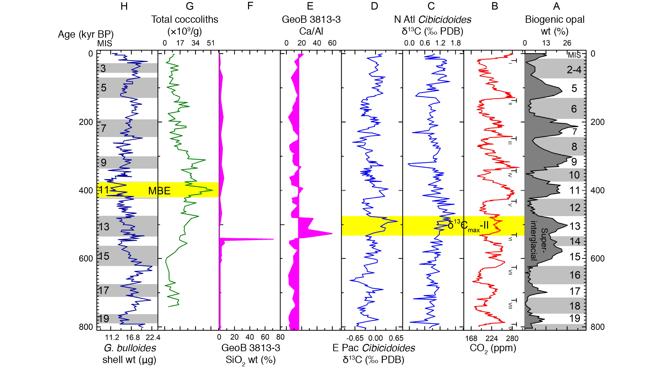
Figure 2: Connection between the δ13Cmax-II and Mid-Brunhes events. (A) Biogenic opal wt % in Core PS28-254, off W. Antarctic (Hillenbrand et al. 2009); (B) Ice-core CO2 (ppm) at EPICA Dome C (Lüthi et al. 2008); (C), (D) Benthic δ13C at ODP 982 and ODP 849 (Barker et al. 2001); (E), (F) Ca/Al ratio and biogenic opal in Core GeoB 3813-3, S. Atlantic, respectively (Gengele and Schimitder 2001); (G) Total coccoliths from ODP 1082, SO; (H) Globigerina bulloides shell weight as dissolution index from ODP 982, N. Atlantic (Barker et al. 2006) |
Figure 2 illustrates how δ13Cmax-II could have led to the MBE via processes in the SO. The event δ13Cmax-II occurred during the younger part of the "super-interglacial" spanning from marine isotope stage (MIS) 15 to 13 (621-478 kyr BP; Fig. 2a-d), associated with a possible collapse of the West Antarctic Ice Sheet (Hillenbrand et al. 2009). The abnormally prolonged stratification in the SO during this period led to a large increase in the abyssal reservoir of Si and other nutrients. Meanwhile, the northward leakage of its Si-rich water to the low-latitude ocean caused a series of biogeochemical events including basin-scale sub-surface diatom blooms in the Southern Atlantic and the accumulation of the vast laminated diatom mat deposits (Fig. 2f). This was followed by coccolithophore blooms when Si was exhausted (Fig. 2e; Gingele and Schmieder 2001). In parallel, the small-sized coccolithophore assemblages began to dominate the global ocean during MIS 15, peaking in MIS 11 and leading to the deep-water carbon dissolution that characterized the mid MBE (Fig. 2g-h; Barker et al. 2006). Therefore, δ13Cmax-II was connected to the MBE by a sequence of events, and probably a similar connection also exists between the δ13Cmax-III and the MPT (Wang et al. 2014).
Since the Earth is currently in a new δ13Cmax, it is crucial to understand the nature of δ13Cmax events and their impacts on the global climate and ocean. This is particularly important for the debates on the next glacial inception (e.g. Berger and Loutre 2002; Müller and Pross 2007). We thus suggest that climate models with a carbon cycle should be used to test hypotheses regarding the dynamics of the carbon cycle in the past on long timescales, which will be crucial for us to improve our long-term future projections.
affiliation
State Key Laboratory of Marine Geology, Tongji University, Shanghai, China
contact
Pinxian Wang: pxwangtongji.edu.cn
references
Archer D et al. (2000) Rev Geophys 38: 159-189
Armstrong RA et al. (2001) Deep-Sea Res Pt II 49: 219-236
Barker S et al. (2006) Quat Sci Rev 25: 3278-3293
Berger A, Loutre MF (2002) Science 297: 1287-1288
Gingele FX, Schmieder F (2001) Earth Planet Sc Lett 186: 93-101
Giorgioni MH et al. (2012) Paleoceanography 27: PA1204
Hillenbrand C-D et al. (2007) Quat Sci Rev 28: 1147-1159
Hodell DA, Venz-Curtis KA (2006) Geochem Geophy Geosy 7: Q09001
Holbourn AE et al. (2007) Earth Planet Sc Lett 261: 534-550
Jiao N et al. (2010) Nat Rev Microbiol 8: 593-599
Kocken IJ et al. (2019) Clim Past 15: 91-104
Lüthi D et al. (2008) Nature 453: 379-382
Ma W et al. (2014) Geo-Marine Letters 34: 541-554
Miller K et al. (1991) J Geophys Res 69: 6829-6848
Müller UC, Pross J (2007) Quat Sci Rev 26: 3025-3029
Pälike H et al. (2006) Science 314: 1894-1898
Tian J et al. (2014) Earth Planet Sc Lett 406: 72-80
Wang P et al. (2004) Paleoceanography 19: A4005
Wang P et al. (2010) Earth Planet Sc Lett 290: 319-330
Matteo Willeit and Andrey Ganopolski
Model simulations reveal the importance of atmospheric CO2 and glacial erosion for Quaternary climate dynamics, in particular for the transition from glacial cycles with a periodicity of 40,000-year to 100,000-year cycles at around 1 million years ago.
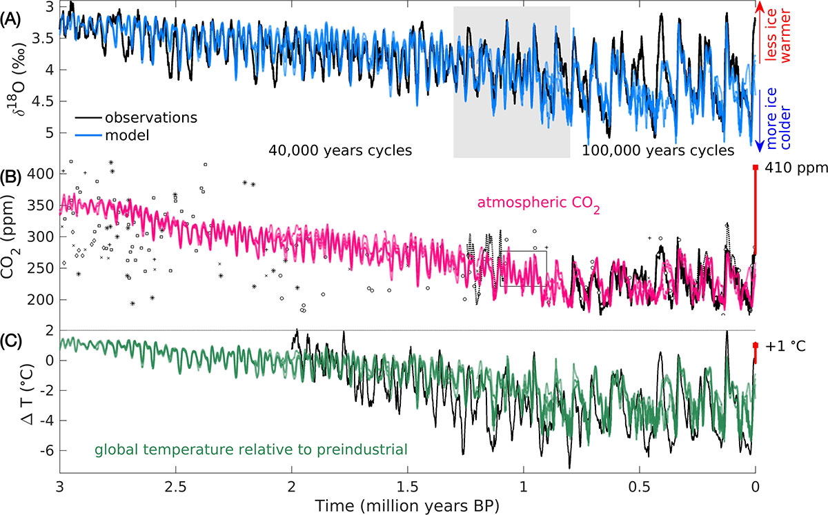
The Quaternary is the most recent geological period, covering the past ~2.6 million years. It is characterized by the presence of glacial-interglacial cycles associated with the cyclic growth and decay of continental ice sheets in the Northern Hemisphere. Climate variations during the Quaternary are best seen in oxygen isotopes measured in deep-sea sediment cores, which represent variations in global ice volume and ocean temperature (Lisiecki and Raymo 2005). These data show clearly that there has been a general trend towards larger ice sheets and cooler temperatures over the last 3 million years, accompanied by an increase in the amplitude of glacial-interglacial variations and a transition from mostly symmetrical cycles with a periodicity of 40,000 years (40 kyr) to strongly asymmetric 100-kyr cycles at around 1 million years ago (Fig. 1a). The ultimate causes of these transitions in glacial cycle dynamics still remain debated.
 |
|
Figure 1: (A) Comparison of modeled and observed (Lisiecki and Raymo 2005) stable oxygen isotopes in deep sediment cores over the last 3 million years. The grey shaded area indicates the period characterized by the transition from glacial cycles with a period of 40 kyr to cycles with a period of 100 kyr. Modeled benthic δ18O is estimated from the modeled sea level, zSL, and deep ocean temperature, Td, as follows: δ18O = 4.0 − 0.22 Td − 0.01 zSL. (B) Modeled atmospheric CO2 concentration compared with ice-core data (solid black line; Bereiter et al. 2015) and various proxy reconstructions (symbols and dotted line, circles: Hönisch et al. 2009; squares: Martínez-Botí et al. 2015; *: Bartoli et al. 2011; + and ×: Seki et al. 2010; diamonds: Badger et al. 2013; black box: Higgins et al. 2015; dotted lines: Chalk et al. 2017). The red line represents the observed CO2 increase since the beginning of the industrial revolution and the red square indicates the observed value at the end of 2018. (C) Modeled global temperature relative to preindustrial compared with reconstructions (Snyder 2016). The red line and square indicate the temperature increase of ~1°C since preindustrial. |
The role of atmospheric CO2 changes in shaping Quaternary climate dynamics is not yet fully understood, largely because of the poor observational constraints on atmospheric CO2 concentrations for the time prior to 800 kyr before present (BP), beyond the period covered by high-quality ice-core data. Proxy-based reconstructions suggest that, over the past ~2 million years, CO2 did not significantly deviate from the range of concentrations measured in ice cores, but that it was substantially higher during the late Pliocene (e.g. Hönisch et al. 2009; Martínez-Botí et al. 2015). A long-term cooling trend associated with a decrease in atmospheric CO2 concentration has been invoked as a possible mechanism to explain the glaciation of Greenland and more generally the Northern Hemisphere at around 3 million years ago (Lunt et al. 2008; Willeit et al. 2015).
It has also been suggested that Northern Hemisphere continents were all covered by thick terrestrial sediments before the Quaternary, an expected outcome of the tens of millions of years that the bedrock was exposed to weathering before the initiation of glacial cycles. The observed present-day sediment distribution, which is characterized by exposed bedrock over large parts of northern North America and Eurasia, is a result of glacial erosion by Quaternary ice sheets. It has been proposed that gradual removal of the sediment layer by glacial erosion could have changed the ice sheets' response to orbital forcing (Clark and Pollard 1998).
Modeling natural climate variability of the past 3 million years
We have used the simplified Earth system model CLIMBER-2 to elucidate the drivers behind the transitions in glacial cycles of the Quaternary (Willeit et al. 2019). Besides the ocean and atmosphere, the model includes a dynamic vegetation module, interactive ice sheets for the Northern Hemisphere, and a fully coupled global carbon cycle, allowing us to interactively simulate atmospheric CO2 (Ganopolski and Brovkin 2017). The model was driven only by changes in the orbital configuration and different scenarios for slowly varying boundary conditions, including CO2 outgassing from volcanoes as a geologic source of CO2, and changes in sediment distribution over the continents. Antarctica is prescribed at its present state in the model, but its effect on sea level is accounted for, to a first approximation, by assuming an additional 10% contribution from Antarctica on top of sea-level variations from simulated changes in Northern Hemisphere ice volume.
When the model is driven by orbital variations and optimal sediment distribution and volcanic outgassing scenarios, it reproduces the evolution of many reconstructed characteristics of Quaternary glacial cycles. It simulates most of the details of the observed oxygen isotope δ18O curve (Fig. 1a), including long-term trends and glacial-interglacial variability. The relative contribution of deep-sea temperature and sea-level variations to δ18O variability changes substantially through time, with temperature variations more important during the early Quaternary, and sea-level variations dominating the signal during the late Quaternary. The model also captures the secular cooling trend of approximately -1°C/million years in sea surface temperatures. The intensification of Northern Hemisphere glaciation after ~2.7 million years ago is marked by a rather abrupt increase in global ice-volume variations and an increase in iceberg flux from the Laurentide ice sheet into the North Atlantic, in good agreement with a proxy for ice-rafted debris. Interglacial atmospheric CO2 concentrations decrease from values of ~350 parts per million (ppm) during the late Pliocene to values between 260 and 290 ppm, typical of the past 800,000 years, at ~1 million years ago (Fig. 1b). The amplitude of glacial-interglacial CO2 variations increases from ~50 ppm at the beginning of the Quaternary to ~80 to 90 ppm during the 100-kyr cycles of the past million years.
Initiation of NH glaciation and transition from 40- to 100-kyr cycles
Our results imply a strong sensitivity of the Earth system to relatively small variations in atmospheric CO2. A gradual decrease of CO2 to values below ~350 ppm led to the start of continental ice-sheet growth over Greenland and more generally over the Northern Hemisphere at the end of the Pliocene and beginning of the Pleistocene, around 2.7 million years ago. Subsequently, the waxing and waning of the ice sheets acted to gradually remove the thick layer of unconsolidated terrestrial sediments that had been formed previously over continents by the undisturbed action of weathering over millions of years. The erosion of this sediment layer – it was essentially bulldozed away by moving glaciers – affected the evolution of glacial cycles in several ways. First, ice sheets sitting on soft sediments are generally more mobile and thinner than ice sheets grounded on hard bedrock, because ice slides more easily over sediments compared to bedrock. This makes ice sheets more vulnerable to increasing summer insolation and thus facilitates their retreat. Additionally, glacial sediment transport to the ice-sheet margins generates substantial amounts of dust that, once deposited on the ice-sheet surface, increases melting of the ice sheets by lowering surface albedo. Model results show that the gradual increase in the area of exposed bedrock over time led to more stable ice sheets, which were less responsive to orbital forcing and ultimately paved the way for the transition to 100-kyr cycles at around 1 million years ago.
Putting the results into present-day and future perspectives
 |
|
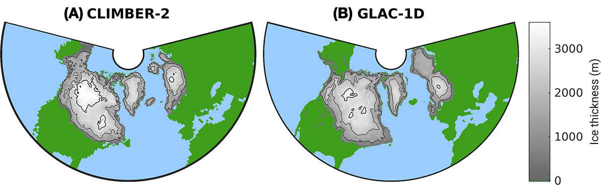
Figure 2: Comparison of the ice-sheet extent and thickness at the Last Glacial Maximum (21 kyr BP) from (A) the CLIMBER-2 model (Willeit et al. 2019) with (B) the model-based reconstruction of Tarasov et al. (2012). |
Our simulations further suggest that global temperature never exceeded the preindustrial value by more than 2°C during the Quaternary (Fig. 1c). Ice-sheet evolution is very sensitive to temperature, and the initiation of Northern Hemisphere glaciation at around 3 million years ago would not have been possible in the model if global temperature were to have been higher than 2°C relative to preindustrial during the early Quaternary. Since the model has been shown to accurately reproduce the sea-level variations over the last 400 kyr and also the spatial ice-sheet distribution at the last glacial maximum (Fig. 2), we are confident that the sensitivity of ice sheets to climate is well represented in the model.
Likewise, our results indicate that the measured CO2 concentration of ~410 ppm at the end of 2018 is unprecedented over the past 3 million years. The climate sensitivity of the model is around 3°C global warming for a doubling of CO2 concentration. This falls in the middle of the current best estimates of climate sensitivity, which range between 1.5 and 4.5°C. It is theoretically possible that the real climate sensitivity is lower than 3°C, in which case the modeled CO2 concentration needed to fit the oxygen isotope record during the early Quaternary would be higher than in the present model simulations, but it would still be unlikely to exceed the present-day value.
In the context of future climate change, our results imply that a failure to significantly reduce CO2 emissions to comply with the Paris Agreement target of limiting global warming well below 2°C will not only bring Earth's climate away from Holocene-like conditions, but also push it beyond climatic conditions experienced during the entire current geological Period, the Quaternary.
affiliation
Potsdam Institute for Climate Impact Research, Germany
contact
Matteo Willeit: willeitpik-potsdam.de
references
Badger MPS et al. (2013) Philos T R Soc A 371: 20130094
Bartoli G et al. (2011) Paleoceanography 26: PA4213
Bereiter B et al. (2015) Geophys Res Lett 42: 542-549
Chalk TB et al. (2017) Proc Natl Acad Sci 114: 13114-13119
Clark PU, Pollard D (1998) Paleoceanography 13: 1-9
Ganopolski A, Brovkin V (2017) Clim Past 13: 1695-1716
Higgins JA et al. (2015) Proc Natl Acad Sci 112: 6887-6891
Hönisch B et al. (2009) Science 324: 1551-1554
Lisiecki LE, Raymo ME (2005) Paleoceanography 20: 1-17
Lunt DJ et al. (2008) Nature 454:, 1102-1105
Martínez-Botí MA et al. (2015) Nature 518: 49-54
Seki O et al. (2010) Earth Planet Sc Lett 292: 201-211
Snyder CW (2016) Nature 538: 226-228
Tarasov L et al. (2012) Earth Planet Sc Lett 315-316: 30-40
Jesse R. Farmer1,2, S.L. Goldstein3,4, L.L. Haynes3,4, B. Hönisch3,4, J. Kim3,4, L. Pena5, M. Jaume-Seguí5 and M. Yehudai3,4
The mid-Pleistocene transition marks the final turn of the Earth system towards repeated major ice ages after ~900,000 years ago. Recent advances in paleoceanographic research provide insight into how ocean processes facilitated the climate changes at that time.
Approximately 900,000 years ago (900 kyr BP), ice ages switched from occurring every 41 kyr to every 100 kyr, lengthening in duration, and strengthening in terms of cooling and ice volume. This "mid-Pleistocene transition" (MPT) occurred without notable changes in Earth's orbit around the sun (i.e. incoming solar radiation). Lacking a defined external trigger, the MPT must represent a fundamental reorganization of Earth's internal climate system, including its greenhouse gas composition, ocean circulation, seawater chemistry, and/or development of more favorable conditions for ice-sheet growth. Recent advances in paleoceanography have made significant progress towards identifying when, how, and why the different components of Earth's climate system changed across the MPT. Here we summarize the biogeochemical insights gleaned from ocean sediments that directly reflect on the global carbon cycle (Fig. 1).
The global climate state of the mid-Pleistocene can be inferred from the benthic foraminiferal oxygen isotope stack of Lisiecki and Raymo (2005) (Fig. 2a), which integrates deep-ocean temperatures and global ice volume. This record shows the MPT as the transition from 41-kyr glacial cycles prior to 1250 kyr BP to dominant 100-kyr glacial cycles by 700 kyr BP (Fig. 2, light blue shading). Within this interval, an anomalously weak interglacial stands out at 900 kyr BP (the "900 ka event"), at the midpoint of what is considered the first 100-kyr glacial cycle (Fig. 2, dark blue shading; Clark et al. 2006).
Proposed explanations for the MPT often invoke declining atmospheric carbon dioxide (CO2) as a fundamental tool to change the climate response to orbital forcing (Clark et al. 2006). Available CO2 reconstructions during this time period are of low temporal resolution but suggest that glacial CO2 decreased by 20-40 ppm sometime between ca. 1000 and ca. 800 kyr BP (Fig. 2b). The ocean most likely caused this CO2 decline via enhanced biological CO2 uptake and/or reduced release of sequestered CO2 back to the atmosphere. General Pleistocene model simulations (Chalk et al. 2017; Hain et al. 2010) highlight three pathways for glacial ocean CO2 sequestration: weaker deep-ocean circulation, increased ocean biological productivity through iron fertilization, and reduced CO2 exchange between deep waters and the ocean surface (broadly termed "stratification"). The common premise behind these pathways is that the missing atmospheric CO2 was trapped in the deep ocean.
Records of ocean circulation
Earlier attempts to reconstruct deep-ocean circulation across the MPT relied on benthic foraminiferal carbon isotope ratios (δ13C). However, regional biology, air-sea gas exchange, and the size of the terrestrial biosphere also impact deep-ocean δ13C, hindering quantitative circulation reconstructions (Lynch-Stieglitz and Marchitto 2014). In contrast, neodymium isotopes (εNd) provide a potentially quantitative approach to separate deep-ocean waters of different geographical origins (Blaser et al. this issue). Distinct εNd values for North Atlantic-sourced and Pacific-sourced deep waters are set by weathering of older and younger continental material into each basin, respectively. In the modern ocean, Nd isotopes behave "quasi-conservatively"; that is, they reflect water-mass mixing, and are not substantially fractionated by biological or physical processes. Moreover, North Atlantic and Pacific end-member εNd values have remained approximately constant over the Pleistocene (Pena and Goldstein 2014).
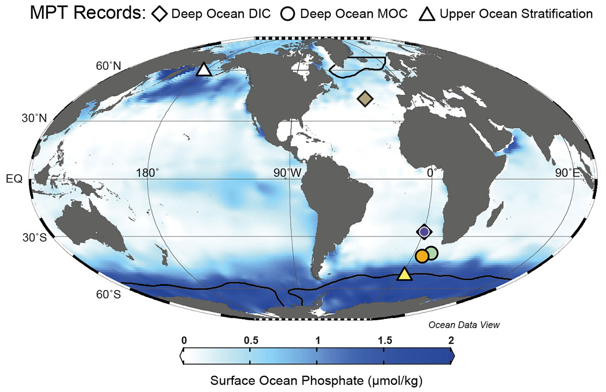 |
|
Figure 1: World map of surface-ocean phosphate concentrations (from GLODAP v2; Lauvset et al. 2016) and core sites of MPT ocean circulation and carbon-cycle reconstructions. A limiting nutrient for ocean productivity, phosphate occurs at high concentrations in areas of the surface ocean where biological consumption of carbon is inefficient, thus limiting ocean uptake of atmospheric CO2. Regions with sufficiently dense surface water to form deep waters (black contour) directly link surface ocean nutrient consumption with deep-ocean circulation and carbon storage. Broadly, enhanced nutrient consumption in these regions lowers atmospheric CO2. Symbols and colors of core locations match data series shown in Figure 2. |
Across the MPT, ocean circulation has been reconstructed from εNd at three South Atlantic locations (Fig. 1; Farmer et al. 2019; Pena and Goldstein 2014). All three records show a dramatic εNd increase following the ca. 950 kyr BP interglacial, indicating reduced North Atlantic deep-water formation and a relatively greater contribution of Pacific-sourced deep water. The elevated εNd values lasted for ca. 100 kyr, right through the ca. 910 kyr BP interglacial (Fig. 2c; Pena and Goldstein 2014). This also marked a transition in glacial deep Atlantic circulation, with weaker circulation (higher εNd) evident in all studied glacials after 950 kyr BP compared to glacials before 950 kyr BP. Intriguingly, this North Atlantic circulation weakening broadly overlaps with the "900 ka event" and the likely period of glacial CO2 decline (Fig. 2a-c).
Ocean impacts on atmospheric CO2
Proxy constraints on ocean-carbon chemistry reveal how weakened ocean circulation may have impacted CO2. Using the elemental ratios B/Ca and Cd/Ca in benthic foraminifera, Lear et al. (2016), Sosdian et al. (2018), and Farmer et al. (2019) observed that glacial deep waters became significantly more "corrosive" (lower carbonate ion concentration) and nutrient-enriched after 950 kyr BP throughout the Atlantic Ocean. Translated to total dissolved carbon, these observations support a ~50 µmol/kg increase during glacials after 950 kyr BP (Fig. 2d), equivalent to a 50 billion ton increase in carbon inventory throughout the deep Atlantic (Farmer et al. 2019). Pairing this information with εNd, Farmer et al. (2019) demonstrated that this deep-ocean carbon accumulation coincided with weakened deep Atlantic Ocean circulation (Fig. 2c-d), suggesting that weaker circulation facilitated accumulation of carbon and other nutrients in the deep Atlantic.
 |
|
Figure 2: Paleoclimatology of the MPT. Brown arrows denote onset and duration of principal changes. Light blue vertical bar denotes MPT interval; dark blue bar denotes interval of the first 100-kyr glacial cycle within the MPT. (A) Benthic oxygen isotope stack (Lisiecki and Raymo 2005); (B) atmospheric CO2 compilation (grey line: Bereiter et al. 2015 compilation; open circles: Higgins et al. 2015; blue and orange filled circles: Dyez et al. 2018 compilation); (C) glacial (filled) and interglacial (open circles) deep Atlantic circulation from εNd (purple: Farmer et al. 2019; light orange/green: Pena and Goldstein 2014); (D) glacial deep Atlantic dissolved inorganic carbon content calculated from benthic foraminifer B/Ca (purple: Farmer et al. 2019; olive: Lear et al. 2016 and Sosdian et al. 2018); (E) Subantarctic Zone (SAZ) iron flux (line) and binned glacial maxima averages (circles) (Martínez-García et al. 2011); (F) density gradient between Antarctic Zone (AZ) surface and deep waters (Hasenfratz et al. 2019). |
The implications of deep Atlantic carbon storage on CO2 are difficult to quantify because no simple equivalence exists between carbon concentration in the deep Atlantic Ocean and atmospheric CO2. In model simulations, the magnitude of CO2 reduction from weaker Atlantic circulation depends upon nutrient consumption in the surface Southern Ocean (Hain et al. 2010); with higher nutrient consumption, CO2 sequestration is strengthened. Martínez-Garcia et al. (2011) reconstructed iron flux to the Subantarctic Southern Ocean, finding that peak glacial iron input increased around the beginning of the MPT (ca. 1250 kyr BP), with integrated glacial iron input increasing more gradually over the MPT (Fig. 2e). If this flux represents bioavailable iron, then increasing Subantarctic iron fertilization across the MPT would have increased ocean CO2 sequestration (Fig. 2e; Chalk et al. 2017; Martínez-García et al. 2011). Addressing the hypothesis of increased stratification, Hasenfratz et al. (2019) reconstructed the glacial density contrast between surface and deep waters in the Antarctic Zone of the Southern Ocean, finding an increased density gradient around 700 kyr BP indicating a stronger halocline and longer surface-ocean residence time (Fig. 2f). This implies that a water-column density barrier to CO2 outgassing in the Southern Ocean strengthened by the end of the MPT.
In summary, three key oceanic pathways for atmospheric CO2 drawdown – deep Atlantic Ocean circulation, Subantarctic iron fertilization, and Southern Ocean stratification – all shifted towards favoring a stronger ocean CO2 sink and reduced atmospheric CO2 across the MPT. Yet all three pathways differ in their timing, and these scenarios are not necessarily exhaustive. For example, Kender et al. (2018) argue for enhanced stratification in the Bering Sea after 950 kyr BP (Fig. 1, white triangle), which may have also amplified oceanic CO2 drawdown.
Thus, evaluating the relative and cumulative CO2 impact of these pathways is an important focus for future MPT research. At the same time, sparse records of key ocean-CO2 pathways across the MPT must be expanded – particularly from the Pacific, which is the largest carbon reservoir in the modern ocean (Fig. 1). High-resolution atmospheric CO2 reconstructions are also needed to constrain the precise timing of MPT CO2 change, especially around 900 kyr BP, and to evaluate the relative importance of different oceanic processes (Fig. 2b). By expanding these proxy applications and integrating available evidence, paleoclimatologists will progress towards a mechanistic understanding of the controls on this crucial window of Earth's climate evolution, encompassing the rise of hominids and the background climate that mankind is altering today.
affiliations
1Department of Geosciences, Princeton University, NJ, USA
2Max-Planck Institute for Chemistry, Mainz, Germany
3Department of Earth and Environmental Sciences, Columbia University, New York, NY, USA
4Lamont-Doherty Earth Observatory of Columbia University, Palisades, NY, USA
5Department of Earth and Ocean Dynamics, University of Barcelona, Spain
contact
Jesse R. Farmer: jesse.farmerprinceton.edu
references
Bereiter B et al. (2015) Geophys Res Lett 42: 542-549
Chalk TB et al. (2017) Proc Natl Acad Sci 114: 13114-13119
Clark PU et al. (2006) Quat Sci Rev 25: 3150-3184
Dyez K et al. (2018) Paleoceanogr Paleocl 33: 1270-1291
Farmer JR et al. (2019) Nat Geosci 12: 355-360
Hasenfratz A et al. (2019) Science 363: 1080-1084
Hain MP et al. (2010) Glob Biogeochem Cy 24: GB40239
Higgins J et al. (2015) Proc Natl Acad Sci 112: 6887-6891
Kender et al. (2018) Nat Commun 9: 5386
Lauvset SK et al. (2016) Earth Syst Sci Data 8: 325-340
Lear CH et al. (2016) Geology 44: 1035-1038
Lisiecki L, Raymo M (2005) Paleoceanography 20: PA1009
Lynch-Stieglitz J, Marchitto TM (2014) Treatise on Geochemistry (2nd Edition): 438-451
Martínez-Garcia A et al. (2011) Nature 476: 312-315
Katrin J. Meissner1,2 and Laurie Menviel1
Climate models are not able to simulate the full extent of atmospheric CO2 rise during the deglaciation. Involved processes are complex and non-linear; improvement could be achieved with better representations of transient ocean circulation changes and more complex parametrizations of ecosystems.
Our planet experienced dramatic changes over the past 20,000 years (kyr), transitioning from full glacial conditions to the current interglacial, the Holocene. During this deglaciation, large Northern Hemispheric ice sheets disintegrated, leading to a global sea-level rise of ~134 m (Lambeck et al. 2014). Changes in biogeochemical cycles on land and in the ocean caused a net release of greenhouse gases into the atmosphere, resulting in a rise of ~90 parts per million (ppm) in CO2, ~300 parts per billion (ppb) in CH4 and ~60 ppb in N2O (Köhler et al. 2017). Marine and terrestrial ecosystems reorganized spatially to adapt to the temperature and precipitation changes that resulted from all of these processes.
These changes did not occur in a continuous or predictable way. The last glacial termination was, on the contrary, quite complex; it was characterized by millennial-scale variability and interhemispheric asynchronies. Like an old flickering fluorescent bulb when switched on, different regions warmed, and cooled again, at different times during the transition. As can be seen in Figure 1, the rise in greenhouse gas concentrations also showed a stepwise behavior, with periods of rapid changes, including CO2 rises of ~13 ppm within 100-200 years (Marcott et al. 2014), and other periods of stagnation or even reversal.
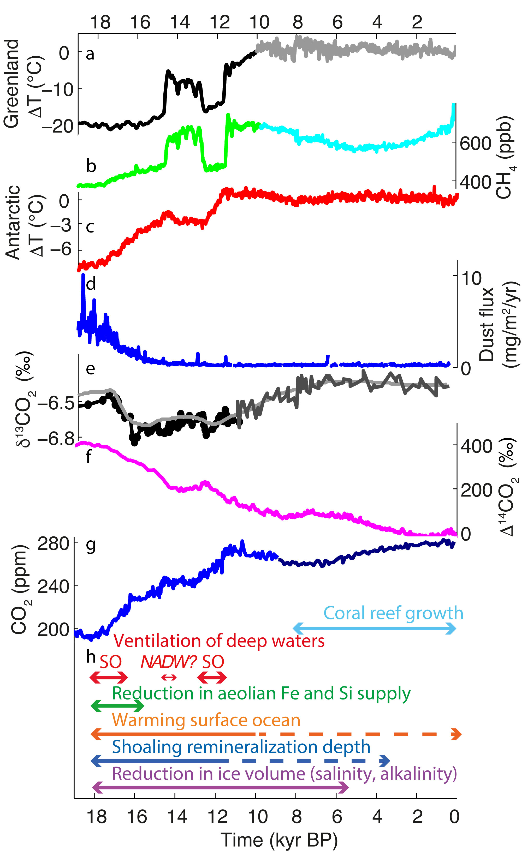 |
|
Figure 1: Timeseries of (A) Greenland surface air temperature anomalies, (B) atmospheric CH4 concentrations, (C) Antarctic surface-air-temperature anomalies, (D) dust flux, (E) δ13CO2, (F) ∆14CO2, (G) CO2, (H) estimated time span of processes discussed in text; SO stands for ventilation of Southern Ocean, NADW for deepening of North Atlantic Deep Water. References are given in the online version of this article (doi.org/10.22498/pages.27.2.60). |
A rather simple math question
While part of the glacial terrestrial carbon on exposed continental shelves was lost due to flooding (182-266 petagram carbon (PgC); Montenegro et al. 2006), CO2 fertilization, generally warmer and wetter conditions, and the newly available land under retrieving ice sheets were conducive to an overall increase in terrestrial carbon during the deglaciation. Recent estimates of net reservoir changes based on global mean ocean δ13C suggest a 300 to 460 PgC increase across the last deglaciation (Menviel et al. 2017), or even higher (~850 PgC; Jeltsch-Thömmes et al. 2019).
To account for the increase in atmospheric CO2, the ocean must therefore have released a total of ~500 to 1050 PgC across the deglaciation, of which ~190 PgC led to the observed increase in atmospheric CO2 and 300 to 850 PgC were fixed on land. How did the ocean pull this off?
There is plenty of carbon in the ocean. The modern ocean is estimated to contain ~38,000 PgC (Ciais et al. 2013), making the glacial-interglacial change a mere 1-3% of reservoir change. This rather small change – from an oceanic point of view – had large effects on the climate system. It was likely caused by a combination of the physical, biological, and chemical processes detailed below (Fig. 2). However, no state-of-the-art climate model has been able to simulate the full amplitude of change so far and the sequence of events is still poorly constrained. We have not (yet) been able to solve our rather simple math problem.
 |
|
Figure 2: Best estimates of processes contributing to atmospheric CO2 changes during the deglaciation. Dark arrows indicate high level of scientific understanding, light arrows indicate medium to low level of scientific understanding. Estimates are discussed in the text or in references in the online version of this article (doi.org/10.22498/pages.27.2.60). |
Physical and chemical processes
Given that CO2 is more soluble in cold than warm water, some of the marine carbon release can be explained by ocean warming during the deglaciation (~+25 ppm; Kohfeld and Ridgwell 2009; Ciais et al. 2013). Melting ice sheets add freshwater to the ocean, decreasing salinity, which would have partly counteracted the temperature solubility effect (~-6 ppm; Kohfeld and Ridgwell 2009). This process also decreases ocean alkalinity and DIC concentrations. Such a decrease in alkalinity decreases the solubility of CO2; however, decreasing alkalinity and DIC at a 1:1 ratio leads to an increase in solubility (~-7 ppm; Kohfeld and Ridgwell 2009). Changes in pressure due to rising sea levels and a decrease in deep-ocean alkalinity would have led to changes in the accumulation/dissolution rates of calcium carbonate in marine sediments, which is a negative feedback, and has a tendency to restore carbonate ion concentrations, and therefore alkalinity. Furthermore, the effect of weathering on land would have led to a small drawdown of atmospheric CO2, mitigated by changes in the carbonate compensation depth.
Biological processes
Some of the surface's dissolved inorganic carbon (DIC) is removed by photosynthesis and transformed into organic carbon. A small percentage of this organic carbon is exported into deeper layers and remineralized into DIC. The strength of this "soft tissue pump" depends on the net primary productivity, which is a function of temperature, nutrient and light availability, competition between species, and the Redfield ratios of the species in question. Nutrient availability depends on ocean circulation and on external fluxes of micronutrients, such as aeolian iron or silica fertilization from dust. For example, the net effect of decreasing dust deposition during the deglaciation has been estimated to have contributed ~+19 ppm to the CO2 rise (Lambert et al. 2015). The strength of the "soft tissue pump" also depends on the remineralization depth of organic carbon. This is a function of the particles' sinking speed and the remineralization rates in the deep ocean. A shoaling of the remineralization depth could have led to a +20 to +30 ppm increase in CO2 (Kwon et al. 2009; Matsumoto 2007; Menviel et al. 2012), but large uncertainties remain.
Calcifying organisms form CaCO3 shells or skeletons in addition to their soft tissue. The calcification process removes alkalinity from surface waters and increases alkalinity at depth upon dissolution. A decrease in surface alkalinity reduces the ability of surface waters to dissolve carbon; this pump has therefore been termed the "carbonate counter pump". Any changes in the competition between calcifying and non-calcifying organisms during the deglaciation, for example due to changes in silicic acid or iron availability, would have changed the strength of the combined biological pump (Matsumoto et al. 2002). In addition, a protective calcite shell changes the sinking speed of particles and thus the remineralization depth. The flooding of continental shelves increased the habitat of calcifying coral reefs, decreasing alkalinity and contributing to the Holocene atmospheric CO2 increase (~+12 ppm; Kohfeld and Ridgwell 2009).
Tying it all together: Ocean circulation
Ocean circulation connects all of the processes mentioned above in a complex way. It transports nutrients to the surface for biological carbon fixation. It also determines the residence time of deep water masses and therefore the total accumulation of remineralized carbon in the deep ocean. While much emphasis has been put on understanding North Atlantic circulation changes (e.g. Ritz et al. 2013; Huiskamp and Meissner 2012), it has recently become clear that the Southern Ocean, where most of surface/deep-water exchange takes place, is likely a more important player. Changes in Southern Ocean circulation can be prompted by changes in winds, sea-ice cover, and meridional density gradients, all of which took place during the deglaciation (Menviel et al. 2018). Finally, the Pacific Ocean is not only the largest ocean basin, it is also characterized by very sluggish circulation and therefore a much higher DIC content than any other ocean basin. Any small increase in ventilation in this basin has the potential to dramatically increase atmospheric CO2 concentrations (Menviel et al. 2014; Rae et al. 2014).
What are the models missing?
Although there has been considerable progress in carbon cycle modeling over the past 20 years, we still do not understand, nor are able to accurately simulate, all of the observed changes during the last deglaciation.
The main culprit is likely an insufficient representation and understanding of changes in ocean circulation. As discussed above, deep water masses are supersaturated in old carbon, holding 100 times more carbon than needed to explain the glacial-interglacial changes. Small circulation changes can result in considerable follow-on effects on ocean-air carbon fluxes.
So far, only models of intermediate complexity have been able to study the sequence of events leading to changes in glacial-interglacial atmospheric CO2. The spatial grids of these models are coarse and do not resolve small-scale processes in the ocean that are potentially important. While they capture the main changes in water masses well enough, they are overall too diffusive. Models that are better skilled in representing physical circulation changes, such as eddy-resolving models, cannot be integrated long enough to even get today's deep ocean circulation into equilibrium, let alone today's marine carbon cycle. Simulating a full transient deglaciation with such models is still far beyond the horizon with today's available computer power. However, these models can be used to test single processes under idealized and fixed boundary conditions.
Another culprit is most certainly the representation of ecosystems in our climate models. These model components are still in their infancy. They are highly simplified, representing the whole complexity of marine life with a few functional types for plankton based on simple equations for population dynamics. Carbon uptake, the sinking speed of particles, and remineralization rates are underconstrained and therefore overtuned (Duteil et al. 2012). It is questionable whether these models' ecosystem sensitivities can be trusted under boundary conditions that are significantly different from present-day conditions.
Finally, none of our state-of-the-art climate models include the whole complexity of sediment feedbacks, which played a non-negligible role during the deglaciation.
How do we solve this?
The proxy community is providing an increasingly coherent picture of deglacial changes. For example, recent high-resolution atmospheric CO2 and isotope records from Antarctic ice cores have highlighted the millennial variability and timing of the deglacial atmospheric CO2 increase and potential source reservoirs (Fig. 1). At the same time, the modeling community is simulating the deglaciation, or parts of it, with models of increasing complexity and higher resolution. The ultimate goal in the not-so-distant future is a transient deglacial modeling framework based on high-resolution models including high-complexity ecosystem models and sediment feedbacks to refine the sequence of the events and processes involved in the deglacial atmospheric CO2 increase.
affiliations
1Climate Change Research Centre, University of New South Wales, Sydney, Australia
2ARC Centre of Excellence for Climate Extremes, University of New South Wales, Sydney, Australia
contact
Katrin Meissner: k.meissnerunsw.edu.au
references
Duteil O et al. (2012) Biogeosciences 9: 1797-1807
Huiskamp WN, Meissner KJ (2012) Paleoceanography 27: PA4296
Jeltsch-Thömmes A et al. (2019) Clim Past 15: 849-879
Köhler P et al. (2017) Earth Syst Sci Data, 9: 363-387
Kwon EY et al. (2009) Nat Geosci 2: 630-635
Lambeck K et al. (2014) P Natl Acad Sci USA 111: 15296-15303
Lambert F et al. (2015) Geophys Res Lett 42: 6014-6023
Marcott SA et al. (2014) Nature 514: 616-619
Matsumoto K et al. (2002) Global Biogeochem Cy 16: 1031
Matsumoto K (2007) Geophys Res Lett 34: L20605
Menviel L et al. (2012) Quat Sci Rev 56: 46-68
Menviel L et al. (2014) Paleoceanography 29: 58-70
Menviel L et al. (2017) Paleoceanography 32: 2-17
Menviel L et al. (2018) Nat Comm 9: 2503
Montenegro A et al. (2006) Geophys Res Lett 20: L08703
Rae JWB et al. (2014) Paleoceanography 29: 645-667
Ritz SP et al. (2013) Nat Geosci 6: 208-212
figure 2
Meissner KJ (2007) Geophys Res Lett 34: L21705
Michael J. Henehan and Hana Jurikova
Boron incorporated in marine biogenic carbonates records the pH of seawater during precipitation. From reconstructing atmospheric CO2 beyond ice-core records to deciphering the ocean's role in storing and releasing carbon, boron is proving to be a vital tool in paleoclimate research.
Around a third of anthropogenic CO2 released to date has been taken up by the ocean. Its future capacity to sequester carbon, however, given potentially dynamic biogeochemical feedbacks, is unclear. Studies of the geological past provide numerous examples of how the ocean regulates and moderates atmospheric CO2 levels. To learn from these, however, we need effective recorders of the ocean's carbonate system. Boron (B)-based proxies – namely B/Ca ratios and the boron isotope (δ11B)-pH proxy applied to marine carbonate archives are among the most promising tools for reconstructing past ocean carbonate chemistry and atmospheric CO2. Here we briefly summarize some of the progress, problems, and prospects in the field.
Chemical basis of boron (B) proxies
In short, B-based proxies rely on the predictable pH-dependent speciation of dissolved B in seawater, between borate ion (B(OH)4-, prevalent at higher pH) and boric acid (B(OH)3, prevalent at lower pH), as shown in Figure 1. The B/Ca proxy works on the assumption that the more of the charged borate ion there is in solution (due to higher pH and lower CO2), the more B will be incorporated into the skeletal CaCO3 of marine calcifiers. The δ11B-pH proxy instead leverages the constant isotope fractionation associated with borate ion and boric acid speciation. This fractionation results in a predictable relationship between the δ11B of borate (the species incorporated into biogenic CaCO3) and pH. This foundation in aqueous chemistry has contributed to the considerable success of B-based proxies to date.
 |
|
Figure 1: (A) The relative abundance of boric acid (in red) and borate ion (blue) changes with pH. (B) A fixed isotope fractionation of ~27‰ (independent of pH) between the two means that the isotopic composition (δ11B) of both species changes predictably with pH. Since borate is incorporated into carbonate, carbonate δ11B reflects the pH of the solution in which it grew. |
The B/Ca proxy
The B/Ca proxy is attractive in that the analytical method is simpler, and it requires less sample material than the δ11B-pH proxy. However, the outlook for this proxy is, at present, mixed. In planktic foraminifera, a host of environmental controls are now known to influence how much of the borate present in solution at any given pH is ultimately incorporated into calcite. These include salinity, ambient phosphorous concentration, light levels, and calcification rate (e.g. Allen and Hönisch 2012; Babila et al. 2014; Henehan et al. 2015; Salmon et al. 2016). Clearly, this complicates the use of B/Ca in planktic foraminifera as a straightforward pH proxy. Indeed, high-profile early applications of the proxy to reconstruct surface-ocean pH and hence atmospheric CO2 (Tripati et al. 2009) have since been shown to have been driven by secondary parameters involved in calculation, rather than the measured B/Ca data itself (Allen and Hönisch 2012). On the other hand, in deep-sea benthic foraminifera strong empirical relationships are observed between B/Ca and bottom-water carbonate saturation (∆[CO32-]; Yu and Elderfield 2007). This has been valuable in tracking the migration of CO2-rich deep-water bodies, and for the most part these reconstructions have been consistent with independent observations (e.g. 14C, δ13C, deep-sea coral δ11B). Collinearity between salinity, phosphorous, and ∆[CO32-] within benthic foraminiferal B/Ca calibration datasets (Henehan 2013), however, means some of the non-carbonate system controls seen in planktic foraminifera could still play a role.
On a more positive note, for all of its documented competing controls, in many geological records B/Ca does appear to behave like a pH proxy. For instance, at the Paleocene-Eocene Thermal Maximum, B/Ca declines in tandem with excursions in δ11B (Penman et al. 2014), suggesting that in some settings planktic foraminiferal B/Ca ratios can be at least qualitatively informative. It is thus premature at this point to discount the proxy entirely.
The boron isotope-pH proxy
Using boron isotopes circumvents many issues associated with B/Ca, allowing for quantitative reconstruction of pH and CO2. For example, diagenetic recrystallisation of fossil CaCO3 may result in loss of B (thus changing B/Ca), but the isotopic composition of the remaining B is unaffected (Edgar et al. 2015). Furthermore, factors like temperature and salinity have no competing effects on δ11B outside of their well-understood quantifiable effect on aqueous B speciation (e.g. Henehan et al. 2016). Most importantly, the dominant control of seawater pH on δ11B has been repeatedly demonstrated. For example, pH reconstructed from the δ11B of core-top deep-sea benthic foraminifera closely matches the pH of the water in which they grew (Rae et al. 2011), indicating the sole incorporation of borate into foraminifera and supporting the chemical foundation of the proxy.
For other calcifiers, although the control of pH on δ11B is clear, skeletal carbonate rarely records the δ11B of ambient seawater borate (δ11Bborate) exactly. Instead, their δ11B reflects a combination of δ11Bborate and a superimposed (typically species-specific) physiologically induced offset, termed a "vital effect". In the case of corals, this vital effect reflects the pH to which the calcifying fluid has been raised, which in turn varies with bulk seawater pH (Venn et al. 2013). In brachiopods and bivalves the situation is perhaps more complex, but their δ11B demonstrably varies with ambient pH (e.g. Jurikova et al. 2019).
In planktic foraminifera – our primary archive of surface-water pH and atmospheric CO2 – vital effects are also ubiquitous (unlike in deep-sea benthic foraminifera). Although we know foraminifera also raise the pH of their internal calcifying fluid (Bentov et al. 2009), thus far the most compelling explanation for species-specific deviations from δ11Bborate is microenvironment alteration (e.g. Henehan et al. 2016). This framework recognizes that planktic foraminifera don’t "see" ambient seawater, but rather a layer of seawater immediately surrounding their shell that is too small for turbulent mixing. It predicts, and indeed explains why, symbiont-bearing foraminifera living in the euphotic zone record higher-than-ambient pH and δ11Bborate: because their photosynthetic symbionts take up CO2 from their microenvironment. Conversely, species living below the euphotic zone, or those that don't host symbionts, are surrounded by seawater that is richer in respired CO2, and hence lower in pH. This also explains the lack of vital effects in deep-sea benthic foraminifera, as their slow metabolic rates mean diffusion can keep pace with release of respired CO2.
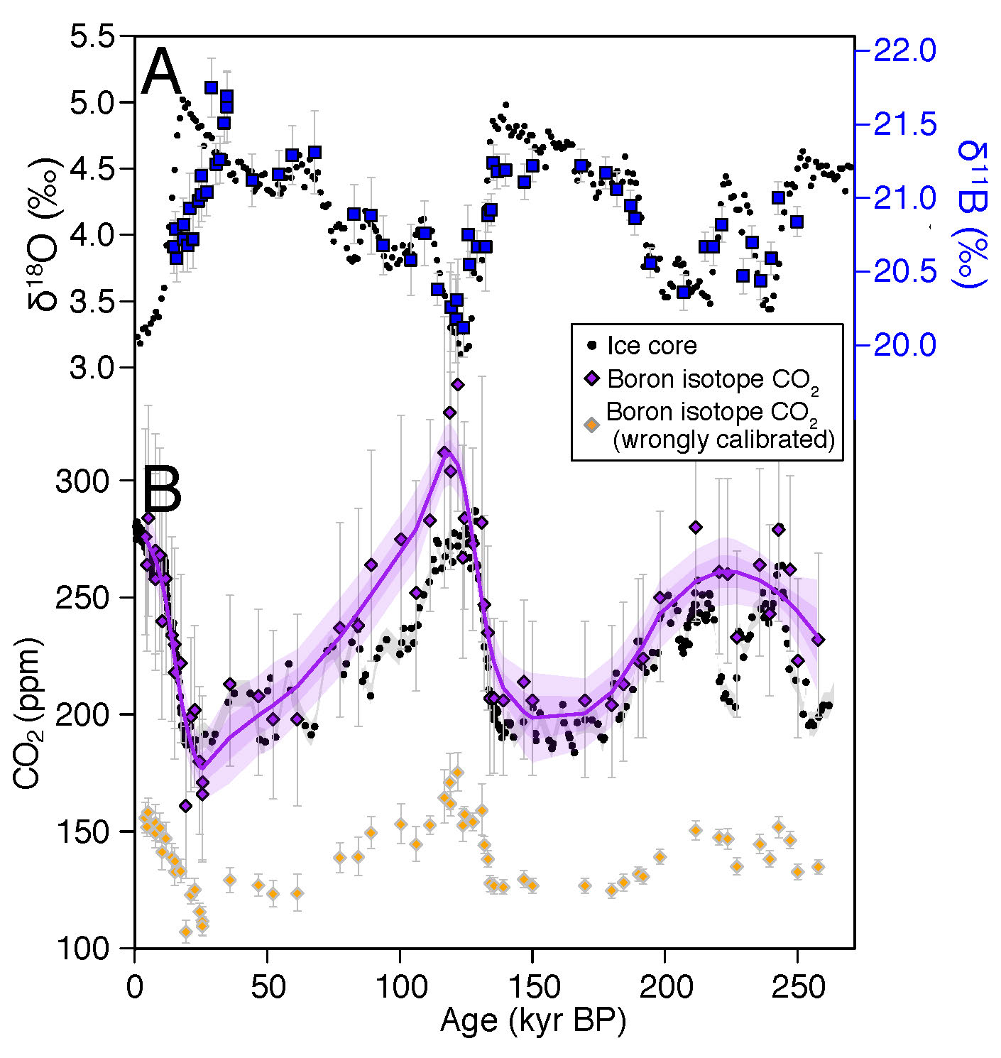 |
|
Figure 2: (A) Foraminiferal (Globigerinoides ruber) δ11B values from Chalk et al. (2017; in blue) covary strikingly well with glacial-interglacial cycles as expressed in benthic foraminiferal δ18O from Lisiecki and Raymo (2005), which in turn reflects global ice volume and deep-sea temperatures. (B) When correctly calibrated for the species' experimentally quantified vital effect, the resulting reconstructed CO2 (violet) is in good agreement with the ice-core composite record from Lüthi et al. (2008; black). (C) However, applying an inappropriate calibration (such as could arise when dealing with extinct species) can lead to spurious CO2 estimates (orange). Here this is illustrated by applying the Orbulina universa calibration of Henehan et al. (2016) to the same G. ruber data. |
Although foraminiferal δ11B clearly varies with pH and CO2 regardless of vital effects (see e.g. data from Chalk et al. 2017 plotted in Fig. 2a), individual species differ significantly in their δ11B-pH (or more commonly δ11Bcalcite-δ11Bborate) calibrations. If a species' calibration is known, pH and CO2 values can be calculated from oligotrophic ocean regions with an accuracy and precision rivaled only by ice cores (Fig. 2b; in purple). However, without a calibration, for example with extinct species, quantifying absolute pH is more challenging. For example, if one erroneously applied a calibration derived for Orbulina universa to these same Globigerinoides ruber data from Chalk et al. (2017; Fig. 2c, in orange), reconstructed CO2 would be inaccurate. Thankfully, efforts to model and constrain vital effects in extinct species are ongoing (e.g. within the SWEET consortium; deepmip.org/sweet); these will reduce this source of uncertainty in deep-time reconstructions.
Beyond reconstructing atmospheric CO2 (by measuring δ11B in planktic foraminifera from regions where the atmosphere and surface ocean CO2 are in equilibrium), the δ11B-pH proxy can also be used to detect transient regional changes in air-sea CO2 disequilibrium. This has elucidated the role of changing ocean carbon storage in driving glacial-interglacial CO2 change, with CO2 release from the deep ocean to the atmosphere now known to have played a major role in pushing the Earth out of the last ice age (e.g. Martínez-Botí et al. 2015; Rae et al. 2018). There is considerable potential for such approaches to be applied in deeper time, for instance to investigate changes in ocean carbon storage during hyperthermal events. Ongoing analytical advances and shrinking sample size requirements mean these sorts of applications are coming into reach, potentially overhauling our understanding of how the ocean has influenced atmospheric CO2 through geological history.
affiliation
German Research Centre for Geosciences (GFZ), Helmholtz Centre Potsdam, Germany
contact
Michael Henehan: michael.henehangfz-potsdam.de
references
Allen KA, Hönisch B (2012) Earth Planet Sc Lett 345–348: 203–211
Babila TL et al. (2014) Earth Planet Sc Lett 404: 67–76
Bentov S et al. (2009) P Natl Acad Sci 106: 21500–21504
Chalk TB et al. (2017) P Natl Acad Sci 114: 13114–13119
Edgar KM et al. (2015) Geochim Cosmochim Acta 166: 189–209
Henehan MJ (2013) PhD thesis, University of Southampton, 348 pp
Henehan MJ et al. (2015) Geochem Geophys Geosystems 16: 1052–1069
Henehan MJ et al. (2016) Earth Planet Sc Lett 454: 282–292
Jurikova H et al. (2019) Geochim Cosmochim Acta 248: 370–386
Lisiecki LE, Raymo M (2005) Paleoceanography 20: PA1003
Lüthi D et al. (2008) Nature 453: 379-382
Martínez-Botí MA et al. (2015) Nature 518: 219–222
Penman DE et al. (2014) Paleoceanography 29: 357-369
Rae JWB et al. (2011) Earth Planet Sc Lett 302: 403–413
Rae JWB et al. (2018) Nature 562: 569–573
Salmon KH et al. (2016) Earth Planet Sc Lett 449: 372–381
Tripati AK et al. (2009) Science 326: 1394–1397
Laura F. Robinson1, G.M. Henderson2, H.C. Ng1 and J.F. McManus3
Despite complex geochemical ocean cycling, sedimentary Pa/Th ratios provide a method for reconstructing past Atlantic overturning rates. This review highlights progress and challenges from the combination of modern and paleo studies.
Measuring rates of processes in the ocean remains a key target in both modern and paleoceanographic studies. Ocean-driven, cross-equatorial heat transport provides a clear physical link between global climate and regional heat distribution, to the extent that constraining the rates of basin-scale meridional overturning circulation is of importance. The decay of radioactive elements (e.g. tritium, radiocarbon) provides a means for quantifying this overturning, given knowledge of isotopic sources and cycling.
In this article we highlight a particular use of radioactive elements within the uranium-series decay chains. The approach relies on the contrasting chemistry of soluble uranium (U) and two daughter elements, thorium (Th) and protactinium (Pa). Specifically, 238U and 235U occur in nature in a fixed ratio, and 238U decays to 230Th (via 234U), while 235U decays to 231Pa. Since uranium resides in seawater sufficiently long to be very well mixed throughout the ocean, the known concentration and predictable decay rates of each isotope can be used to calculate the production of 230Th and 231Pa. These isotopes are therefore produced with a fixed activity ratio of 0.093. Both daughter isotopes are rapidly adsorbed, or "scavenged", onto marine particles, which subsequently accumulate on the seafloor as sediments. Thorium is scavenged more efficiently than Pa by most types of marine particles, leading to contrasting residence times in seawater, allowing for differential lateral transport and measurable shifts in the Pa/Th activity ratio of underlying sediments. These deviations from the production ratio reflect a balance between scavenging and export from the basin via the overturning circulation. Today, the sediments of the North Atlantic have a Pa/Th ratio of ~0.05 because some Pa is being transported southwards and buried in the Southern Ocean (Yu et al. 1996). This export can also be deduced from analyses of seawater Pa and Th concentrations (Deng et al. 2018, as summarized in Fig. 1). In principle, less water advection should result in less export and therefore enhanced burial of Pa, and higher sedimentary Pa/Th ratios in the North Atlantic.
 |
|
Figure 1: This overview figure reproduced from Deng et al. (2018) shows fluxes of 230Th (blue arrows) and 230Th (blue boxes) and 231Pa (yellow arrows) at three latitudes in the Atlantic. When compared to the total production of 230Th (blue boxes) and 231Pa (yellow boxes) these fluxes indicate that only 4% of the 230Th (blue boxes) and 230Th, but 26% of the 231Pa, produced in the North Atlantic are exported southward by ocean circulation in the modern ocean (Deng et al. 2018). It is this relatively larger export of 231Pa on which the Pa/Th proxy for past circulation relies. |
The use of sedimentary Pa/Th ratios to assess past flow was pioneered in 1996 by Yu et al. who compared Holocene and Last Glacial Maximum sediments from across the Atlantic to test whether there was any change in this ratio associated with the cold, glaciated climate. Surprisingly, the results showed very little difference between modern and glacial overturning in the deep ocean. By contrast, Pa/Th analyzed in rapidly accumulating sediments from the Bermuda Rise indicated that there may have been rather large changes in circulation during the deglaciation (McManus et al. 2004). From modestly increased glacial values, suggesting persistent overall overturning, Pa/Th ratios increased markedly to high values close to the production rate during Heinrich Stadial 1, and to elevated values during the Younger Dryas – interpreted as a reduction in overturning strength. Importantly, these changes occurred in association with North Atlantic iceberg discharge events and northern cooling, pointing to a link between freshwater, climate, and reduced Atlantic overturning. The Bermuda Rise Pa/Th record is now widely used as an archetype circulation record for the North Atlantic, providing a modeling target and general reference curve for many paleoclimate studies (e.g. Liu et al. 2009). Similar associations between climate change and changes in sedimentary Pa/Th have been observed throughout the last glacial and deglaciation in the North Atlantic (Gherardi et al. 2005; Böhm et al. 2015; Henry et al. 2016; Lippold et al. 2009; Ng et al. 2018).
Challenges
The complex geochemical cycling of the uranium-series isotopes adds multiple complications to the use of Pa/Th as a circulation tracer. For example, it has been established that Pa is scavenged more effectively onto opal than it is onto carbonates (e.g. Chase et al. 2002; Luo and Ku 2004). Particle concentration and iron-rich phases are other factors that influence the scavenging efficiency of Pa and Th, so Pa/Th could potentially be affected by changes in productivity, nepheloid layers, or hydrothermal activity (e.g. Bradtmiller et al. 2007; Hayes et al. 2015). Recent paleoclimate studies have assessed both the opal concentration and particle flux rates to investigate their competing influence on sedimentary Pa/Th ratios. For example, Bradtmiller et al. (2014) drew on the approach of Yu et al. (1996) to look at spatial patterns of Atlantic sedimentary Pa/Th in three time-slices, filtering for both opal and particle flux. The average of the North Atlantic data supported the early conclusion of Yu et al. (1996), with no significant difference between modern values and those during the Last Glacial Maximum, although spatial and depth differences were apparent. By contrast, the Pa/Th ratio was higher for Heinrich Stadial 1 sediments, consistent with a slowdown in the overall meridional overturning circulation during that time of cold conditions in the North Atlantic.
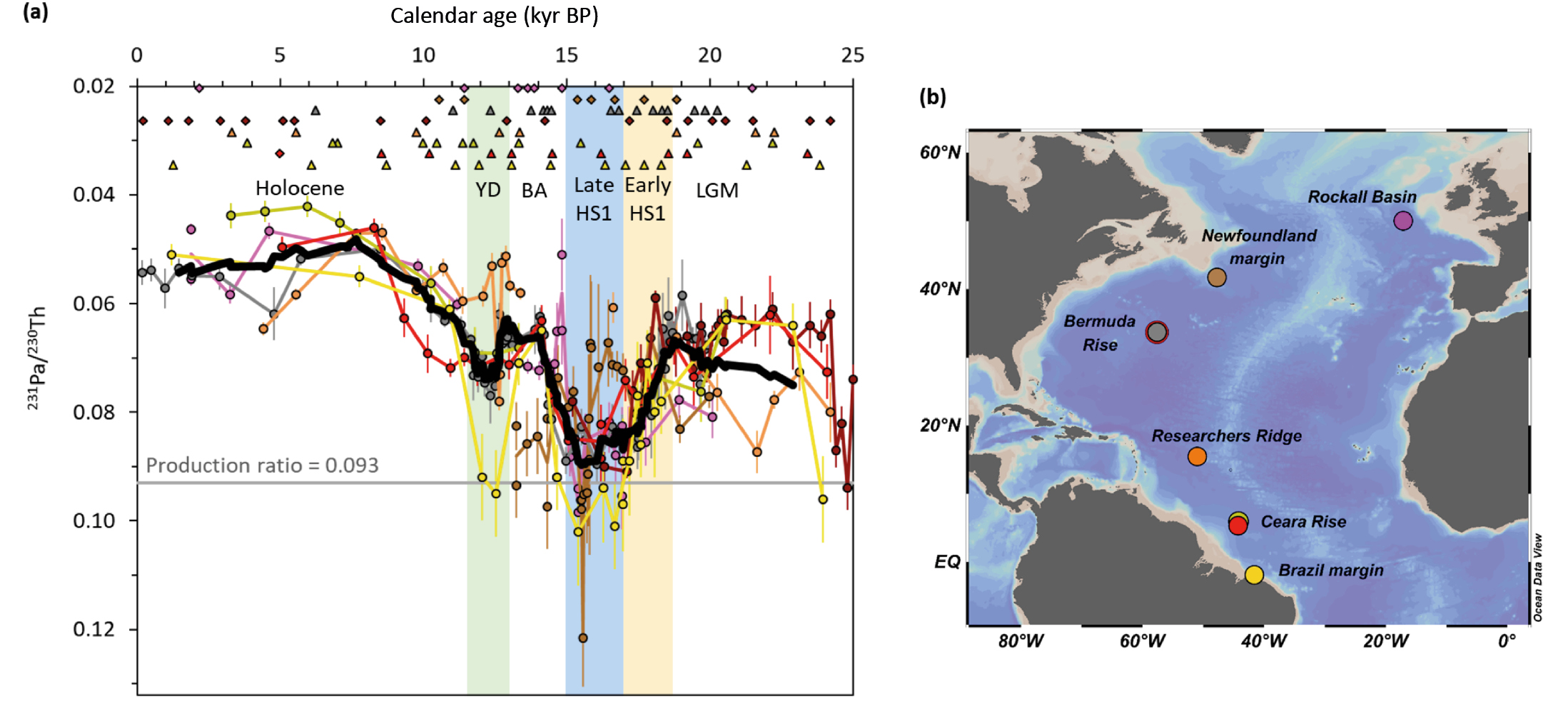 |
|
Figure 2: Past changes in AMOC rate over the last 25,000 years. (A) Compilation of selected Atlantic sedimentary 231Pa/230Th records (Ng et al. 2018). Bold black line is the composite 231Pa/230Th record that reflects the average basin-scale changes in circulation rate (Ng et al. 2018); colors correspond to sites identified in (B) site map. Error bars represent two standard errors of the mean. Triangle and diamond symbols respectively signify 14C and non-14C chronological tie-points. Annotations of key climate events: LGM: Last Glacial Maximum; HS1: Heinrich Stadial 1; BA: Bølling-Allerød; YD: Younger Dryas (Ng et al. 2018). |
Modern observations
Important to the principle of using Pa/Th as a tracer for circulation is the deduction that the scavenging of both isotopes is reversible. Both isotopes generally increase in concentration with depth in the ocean, in both dissolved and particulate phases. Bacon and Anderson (1982) explained this behavior with a simple one-dimensional reversible scavenging model. Over the following decades, analysis of additional seawater profiles led to development of more complicated scavenging models with an "advection" component allowing for a quantification of timescales for Atlantic overturning rates ranging from decades to centuries (Moran et al. 2001). A dramatic increase in the number of seawater analyses, modeling studies, and understanding of Pa/Th in the ocean comes from the ongoing international GEOTRACES program (Schlitzer et al. 2018). Although this greater spatial coverage has enabled broadscale estimates of the export of Pa and Th from the Atlantic (e.g. Fig 1; Deng et al. 2018), the expected pattern of a Pa/Th evolution towards higher values as waters travel along the advective pathways of the Atlantic is not apparent in seawater data. These data suggest that there are aspects of the marine chemistry of Pa and Th that are not yet fully understood, and will require further investigation into their sources, sinks, and cycling. Without this understanding, it is challenging to interpret Pa/Th data from a single location. It remains the case, though, that with sufficient cores to characterize the sedimentary ratio of Pa/Th at a basin scale, the net export of Pa can provide powerful information about advection from the basin. A remaining difficulty in this respect, however, is to robustly interpret sediment data at times when water-mass proxies (e.g. δ13C, Cd/Ca) indicate that there was deep-water flow both into and out of the North Atlantic.
Assessing the basin-scale behavior of Pa/Th in such situations is an important target of ongoing modeling efforts. Early efforts to simulate the behavior of Pa/Th in the Atlantic confirmed its potential sensitivity to changes in overturning circulation rates, including on millennial timescales (Marchal et al. 2000). A subsequent study utilized an inverse method to place constraints on the departures from the observed modern circulation constrained by relatively limited sedimentary data (Burke et al. 2011). More recently, the direct incorporation of Pa and Th in ocean circulation models (e.g. Missiaen et al. 2019) heralds new possibilities for insights derived from comparisons of simulations with both water-column and sedimentary data.
Where are we now?
Despite challenges, there is a clear place for the use of sedimentary Pa/Th in the reconstruction of past circulation rates. By using multiple cores, and by assessing the potential complicating factors from variable scavenging rates, Pa/Th can act as a powerful proxy. Indeed, a recent synthesis of Atlantic deglacial sedimentary cores, filtered for particle and opal flux, yields a coherent pattern over the last 25,000 years (Fig. 2; Ng et al. 2018). In particular, cores from the deep high-latitude North and the West Atlantic all yield broadly similar results as the original high-resolution Bermuda Rise records, emphasizing a strong case for a broad overturning control on the sedimentary Pa/Th ratio, with links to past millennial climate events.
With closer integration of GEOTRACES seawater and core-top sediment data with modeling there is scope to move from general statements on overall overturning rates to a more nuanced interpretation. While quantifying overturning rates may remain challenging, drawing on the strength of these intriguing isotopes has the potential to continue to reveal new information on how and why the oceans have changed in the past.
affiliations
1School of Earth Sciences, University of Bristol, UK
2Department of Earth Sciences, University of Oxford, UK
3Lamont-Doherty Earth Observatory, Columbia University, Palisades, NY, USA
contact
Laura F. Robinson: Laura.Robinsonbristol.ac.uk
references
Bacon M, Anderson R (1982) J Geophys Res 87: 2045-2056
Böhm E et al. (2015) Nature 517: 73-76
Bradtmiller LI et al. (2007) Paleoceanography 22: PA4216
Bradtmiller LI et al. (2014) Nat Commun 5: 5817
Burke A et al. (2011) Paleoceanography 26: PA1212
Chase Z et al. (2002) Earth Planet Sc Lett 204: 215-229
Deng F et al. (2018) Biogeosciences 15: 7299-7313
Gherardi JM et al. (2005) Earth Planet Sc Lett 240: 710-723
Hayes CT et al. (2015) Deep-Sea Res Pt II 116: 29-41
Henry LG et al. (2016) Science 353: 470-474
Lippold J et al. (2009) Geophys Res Lett 36: L12601
Liu Z et al. (2009) Science 325: 310-314
Luo SD, Ku TL (2004) Earth Planet Sc Lett 220: 201-211
Marchal O et al. (2000) Paleoceanography 15: 625-641
McManus JF et al. (2004) Nature 428: 824-837
Missiaen L et al. (2019) Clim Past Discuss
Moran SB et al. (2001) Geophys Res Lett 28: 3437-3440
Ng HC et al. (2018) Nat Commun 9: 2947
Patrick Blaser1, M. Frank2 and T. van de Flierdt3
The dissolved neodymium isotope composition of seawater is widely used to study past changes in provenance and mixing of different water masses in the ocean. We discuss mechanisms controlling signal formation and preservation, proxy strengths, and current challenges.
The samarium-neodymium (Nd) decay system has been widely used to determine the age of crustal rocks and the provenance of detrital sediments. However, the dissolved radiogenic isotope composition of Nd (expressed as εNd = [(143Nd/144Nd)/0.512638 – 1] × 104) in seawater also traces the distribution of major water masses and their mixing. This is the foundation for using Nd isotopes as a tracer for ocean circulation (van de Flierdt et al. 2016).
Disentangling ocean circulation from carbon storage
For decades, the reconstruction of past ocean circulation relied on the stable isotope composition of the nutrient component carbon (C) in marine calcareous organisms (13C/12C ratio expressed as δ13C; Fig. 1). However, both biological cycling and ocean circulation play major roles in setting the measured δ13C signature. In contrast, the lithogenic element Nd is not actively involved in marine biological cycling. Recorded in and extracted from oceanic archives, radiogenic Nd isotopes fingerprint where a water mass acquired its Nd isotope signature. Thus, the combination of Nd and C isotopes in oceanic archives allows us to disentangle deep ocean circulation from carbon storage under past climatic conditions and becomes more valuable than the sum of its parts.
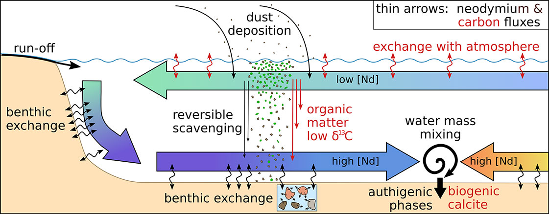 |
|
Figure 1: Simplified scheme of the most relevant biogeochemical processes influencing Nd and C isotope compositions of water masses; from surface water via deep end-member formation to mixing and archiving. Large arrows represent water masses with colors qualitatively implying different isotope compositions. |
For example, Piotrowski et al. (2005) combined Nd, oxygen, and carbon isotopes from a high sedimentation site in the South Atlantic to show that glacial-interglacial transitions first manifested themselves in changes in ice sheets, followed by ocean carbon storage, and finally ocean circulation. Pena and Goldstein (2014) extended the εNd record across the mid Pleistocene and found that Atlantic meridional overturning skipped a beat during interglacial marine isotope stage 23 (approximately 900 kyr BP), increasing carbon sequestration and thereby promoting ice-sheet build-up and setting the stage for the mid-Pleistocene transition. During this period, glacial cycles switched from a 41 kyr periodicity to one of 100 kyr (see also Farmer et al. this issue). For the Last Glacial Maximum, Howe et al. (2016a) compiled Atlantic εNd data suggesting that southern sourced water was less prevalent than inferred from carbon isotopes. This implies that biological cycling must have played a greater role than previously thought. These examples demonstrate the value of seawater derived εNd as a water-mass proxy in the paleoceanographer’s toolbox.
What determines the seawater Nd isotope signal?
Lithogenic in origin, dissolved Nd is introduced into surface waters by erosion and weathering of continental crust. Hence, water masses typically acquire their Nd isotope fingerprint at the interface with continents. Subsequently, convection leads to the export of these characteristic εNd signatures to deep waters (Fig. 1).
The mean residence time of Nd in the deep oceans is on the order of centuries, and is thus similar to the mean ocean overturning time. This similarity of time constants is the decisive factor rendering εNd a suitable tracer for ocean water masses. Hence, εNd behaves largely conservatively away from ocean margins (no significant sources or sinks), with measured signatures primarily reflecting the mixture of distinct water masses transported across ocean basins (Fig. 2a). On regional and local scales, however, geochemical processes can modulate the residence time of Nd dissolved in seawater.
The concentration of dissolved Nd generally increases with water depth, indicating a combined control of advection and vertical transport via adsorption and desorption from particles. This can transfer Nd vertically through the water column and across water-mass boundaries. At the ocean bottom, fluxes of Nd across the sediment-seawater interface have been observed both into and out of bottom waters (Haley et al. 2017). In general, such benthic exchange depends on the reactivity of detrital material releasing Nd in the sediment. Exchange may also be facilitated within benthic nepheloid layers through the availability of large particle surface areas (van de Flierdt et al. 2016).
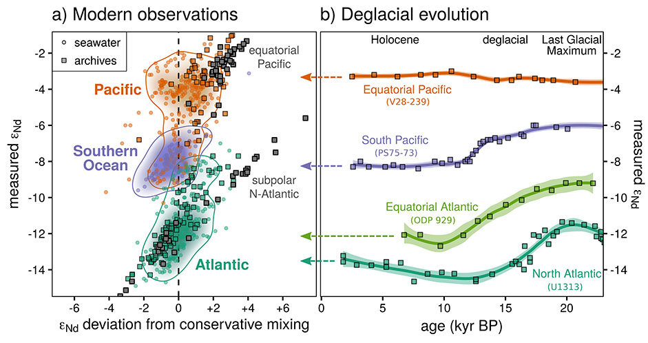 |
|
Figure 2: (A) Measured εNd of seawater and "young" archives (>1500m depth) vs. their deviation from purely conservative mixing of water-mass end-members (Tachikawa et al. 2017). Pacific εNd values are high due to ubiquitous young volcanic rocks, whereas old terranes around the North Atlantic lead to low εNd. The Southern (and Indian) Ocean exhibits intermediate signatures. (B) The εNd evolution from four representative deep sites since the Last Glacial Maximum (Basak et al. 2018; Howe et al. 2016b; Hu and Piotrowski 2018; Lippold et al. 2016; Pöppelmeier et al. 2018). Higher glacial εNd in the Atlantic is generally interpreted to indicate the presence of more Pacific-sourced water, but uncertainties in past end-member εNd and Nd concentrations complicate such interpretations. |
Geochemical processes are not necessarily restricted to regions where water masses are formed and their end-member characteristics are defined. Therefore, a non-conservative element is added to the distribution of εNd in seawater. Ultimately, it is the balance of physical water-mass advection (conservative component) and geochemical processes (non-conservative component) that determines the residence time of dissolved Nd in seawater and whether its isotope composition primarily reflects water-mass mixing. In environments in which exchange processes lead to faster replacement of Nd than water-mass transit, εNd may even be applicable as a kinematic proxy, as Du et al. (2018) suggested for the North Pacific.
What do the archives tell us?
Marine archives record the local Nd isotope signatures of water-mass mixtures. The extraction of unaltered past seawater εNd is challenging but has been achieved from fossil fish debris, deep-sea coral skeletons, and ferromanganese deposits in the form of crusts, nodules, and coatings on bulk sediment particles and inside foraminiferal calcite tests (Fig. 2a).
However, the early diagenetic archiving process is currently not well understood and in some regions all attempts to extract local bottom water εNd from core-top sediments have failed (see gray indicated regions in Fig. 2a). The archiving processes comprise co-precipitation of Nd with iron-manganese oxyhydroxides, diffusion into biogenic apatite, and the precipitation in microbially mediated microenvironments. Hence, for sedimentary εNd signatures, one possible explanation for discrepancies compared to seawater εNd is that a pore-water signal is recorded, which itself can reflect a mixture of bottom water and detrital εNd. Pore waters and sedimentary authigenic phases could thus carry additional information about the strength of past benthic exchange (Du et al. 2016).
Improving Nd isotope-based reconstructions of water masses
Mechanisms and magnitudes of Nd supply to the oceans via particles, reactive sediments, or in dissolved form can vary as a function of climatically controlled parameters such as precipitation or ice and vegetation cover on the continents. Thus, the accuracy of εNd as a paleo water-mass proxy often depends on the knowledge of past end-member characteristics (Fig. 2b; Howe et al. 2016a; Pöppelmeier et al. 2018), the impact of non-conservative processes (Blaser et al. 2019), and the fidelity of the archive and extraction method used (Blaser et al. 2016; Du et al. 2016).
Paleoceanographic reconstructions from settings with little input of reactive detritus and expected large water mass fluxes will be least affected by such uncertainties, and interpretations will ideally be based on εNd gradients between different sites. Better data coverage within and near regions of significant benthic exchange and end-member formation, as well as incorporation of Nd concentrations and εNd in ocean circulation models will be important steps to gain deeper insights into past oceanic Nd cycling and water mass circulation. The combination of several tracers can eliminate uncertainties of individual proxies. At the same time a better understanding of present-day Nd cycling through measurements along ocean sections and dedicated process studies at key locations, currently performed as part of the international GEOTRACES program (geotraces.org), will increase the reliability of interpretations based on Nd isotopes.
affiliations
1Institute of Earth Sciences, Heidelberg University, Germany
2GEOMAR Helmholtz Centre for Ocean Research Kiel, Germany
3Department of Earth Science and Engineering, Imperial College London, UK
contact
Patrick Blaser: patrick.blasergeow.uni-heidelberg.de
references
Basak C et al. (2018) Science 359: 900-904
Blaser P et al. (2016) Chem Geol 439: 189:204
Blaser P et al. (2019) Geochim Cosmochim Acta 245: 79-97
Du J et al. (2016) Geochim Cosmochim Acta 193: 14-35
Du J et al. (2018) Nat Geosci 11: 749-755
Haley BA et al. (2017) Front Mar Sci 4: 426
Howe JNW et al. (2016a) Nat Commun 7: 11765
Howe JNW et al. (2016b) Geology 44: 831-834
Hu R, Piotrowski AM (2018) Nat Commun 9: 4709
Lippold J et al. (2016) Earth Planet Sc Lett 445: 68-78
Pena LD, Goldstein SL (2014) Science 345: 318-322
Piotrowski AM et al. (2005) Science 307: 1933-1938
Pöppelmeier F et al. (2018) Paleoceanogr Paleocl 33: 530-543
Tachikawa K et al. (2017) Chem Geol 457: 131-148
van de Flierdt T et al. (2016) Philos T R Soc A 374: 20150293